Preprocesamiento y Creación de Modelos de clasificación#
import warnings
warnings.filterwarnings('ignore')
Preprocesamiento#
import pandas as pd
import numpy as np
from tqdm import tqdm
from keras.preprocessing.text import Tokenizer
tqdm.pandas(desc="progress-bar")
from gensim.models import Doc2Vec
from sklearn import utils
from sklearn.model_selection import train_test_split
from keras_preprocessing.sequence import pad_sequences
from gensim.models.doc2vec import TaggedDocument
import re
import nltk
from nltk.corpus import stopwords
from bs4 import BeautifulSoup

df = pd.read_csv('https://raw.githubusercontent.com/lihkir/Data/main/spam_text_class.csv',delimiter=',',encoding='latin-1')

df = df[['Category','Message']]

df = df[pd.notnull(df['Message'])]

# quitar etiquetas html

def cleanText(text):
    text = BeautifulSoup(text, "lxml").text
    text = re.sub(r'\|\|\|', r' ', text)
    text = re.sub(r'http\S+', r'<URL>', text)
    text = text.lower()
    text = text.replace('x', '')
    return text

df['Message'] = df['Message'].apply(cleanText)
train_test split
max_fatures = 500000

MAX_SEQUENCE_LENGTH = 50

tokenizer = Tokenizer(num_words=max_fatures, split=' ', filters='!"#$%&()*+,-./:;<=>?@[\]^_`{|}~', lower=True)
tokenizer.fit_on_texts(df['Message'].values)

X = tokenizer.texts_to_sequences(df['Message'].values)
X = pad_sequences(X, maxlen=MAX_SEQUENCE_LENGTH)

Y = pd.get_dummies(df['Category']).values

X_train, X_test, y_train, y_test = train_test_split(X,Y, test_size = 0.15, random_state = 42)
SMOTE#
from imblearn.over_sampling import SMOTE

# Crear una instancia de SMOTE
smote = SMOTE(random_state=42)

y_for_smote = np.argmax(y_train, axis=1)

# Aplicar SMOTE al conjunto de entrenamiento
X_train_smote, y_for_smote = smote.fit_resample(X_train, y_train)

# Get unique values in the array
unique_values = np.unique(y_for_smote)

# Initialize one-hot encoded array with zeros
y_train_smote = np.zeros((len(y_for_smote), len(unique_values)))

# Fill in the one-hot array based on the original binary array
for i, value in enumerate(y_for_smote):

    y_train_smote[i, np.where(unique_values == value)] = 1
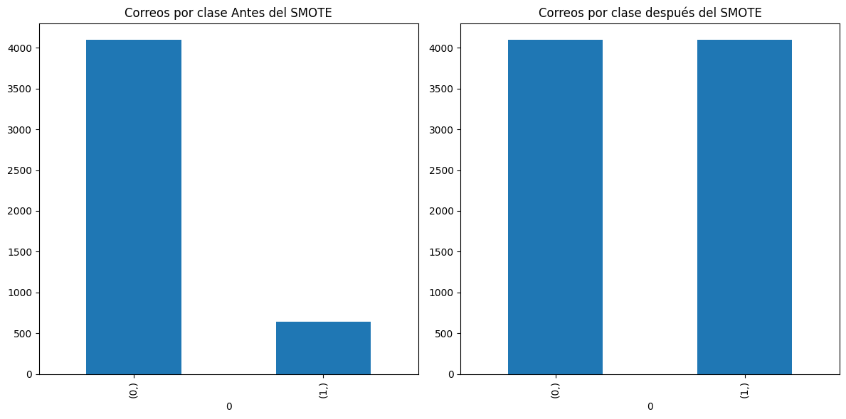
import matplotlib.pyplot as plt

plt.figure(figsize=(12, 6))

# Chart 1
plt.subplot(1, 2, 1)
pd.DataFrame(np.argmax(y_train, axis=1).astype(str)).value_counts().plot(kind='bar', title='Correos por clase Antes del SMOTE')

# Chart 2
plt.subplot(1, 2, 2)
pd.DataFrame(np.argmax(y_train_smote, axis=1).astype(str)).value_counts().plot(kind='bar', title='Correos por clase después del SMOTE')

plt.tight_layout()  # To ensure proper spacing between subplots
plt.show()
Creación y Comparación de Modelos#
LSTM#
train, test = train_test_split(df, test_size=0.000001 , random_state=42)

def tokenize_text(text):
    tokens = []
    for sent in nltk.sent_tokenize(text):
        for word in nltk.word_tokenize(sent):
            if len(word) <= 0:
                continue
            tokens.append(word.lower())
    return tokens

train_tagged = train.apply(lambda r: TaggedDocument(words=tokenize_text(r['Message']), tags=[r.Category]), axis=1)

test_tagged = test.apply(lambda r: TaggedDocument(words=tokenize_text(r['Message']), tags=[r.Category]), axis=1)

d2v_model = Doc2Vec(dm=1, dm_mean=1, vector_size=20, window=8, min_count=1, workers=1, alpha=0.065, min_alpha=0.065)

d2v_model.build_vocab([x for x in tqdm(train_tagged.values)])

for epoch in range(30):
    d2v_model.train(utils.shuffle([x for x in tqdm(train_tagged.values)]), total_examples=len(train_tagged.values), epochs=1)
    d2v_model.alpha -= 0.002
    d2v_model.min_alpha = d2v_model.alpha
100%|██████████| 5571/5571 [00:00<?, ?it/s]
100%|██████████| 5571/5571 [00:00<00:00, 929010.32it/s]
100%|██████████| 5571/5571 [00:00<?, ?it/s]
100%|██████████| 5571/5571 [00:00<00:00, 506326.63it/s]
100%|██████████| 5571/5571 [00:00<00:00, 369547.17it/s]
100%|██████████| 5571/5571 [00:00<?, ?it/s]
100%|██████████| 5571/5571 [00:00<?, ?it/s]
100%|██████████| 5571/5571 [00:00<00:00, 356228.73it/s]
100%|██████████| 5571/5571 [00:00<?, ?it/s]
100%|██████████| 5571/5571 [00:00<?, ?it/s]
100%|██████████| 5571/5571 [00:00<00:00, 355973.67it/s]
100%|██████████| 5571/5571 [00:00<00:00, 356614.74it/s]
100%|██████████| 5571/5571 [00:00<00:00, 356505.92it/s]
100%|██████████| 5571/5571 [00:00<?, ?it/s]
100%|██████████| 5571/5571 [00:00<?, ?it/s]
100%|██████████| 5571/5571 [00:00<?, ?it/s]
100%|██████████| 5571/5571 [00:00<00:00, 308671.96it/s]
100%|██████████| 5571/5571 [00:00<?, ?it/s]
100%|██████████| 5571/5571 [00:00<?, ?it/s]
100%|██████████| 5571/5571 [00:00<?, ?it/s]
100%|██████████| 5571/5571 [00:00<00:00, 319397.30it/s]
100%|██████████| 5571/5571 [00:00<00:00, 294050.99it/s]
100%|██████████| 5571/5571 [00:00<00:00, 356473.29it/s]
100%|██████████| 5571/5571 [00:00<?, ?it/s]
100%|██████████| 5571/5571 [00:00<00:00, 1231045.13it/s]
100%|██████████| 5571/5571 [00:00<00:00, 356723.62it/s]
100%|██████████| 5571/5571 [00:00<00:00, 356098.44it/s]
100%|██████████| 5571/5571 [00:00<00:00, 336828.51it/s]
100%|██████████| 5571/5571 [00:00<?, ?it/s]
100%|██████████| 5571/5571 [00:00<00:00, 10733333.75it/s]
100%|██████████| 5571/5571 [00:00<?, ?it/s]
Numero de palabras totales que queda en vector de embeddings
len(d2v_model.wv.index_to_key)
9363
top 10 parabras mas similares a ‘urgent’
d2v_model.wv.most_similar(positive=['urgent'], topn=10)
[('aint', 0.754719078540802),
 ('cherish', 0.753497302532196),
 ('pee', 0.7372303605079651),
 ('plate', 0.7127653956413269),
 ('09066612661', 0.7108734250068665),
 ('09061213237', 0.7107982635498047),
 ('wrld', 0.7033034563064575),
 ('pig', 0.7011724710464478),
 ('zogtorius', 0.6995012164115906),
 ('lower', 0.6984557509422302)]
from keras.models import Sequential
from keras.layers import LSTM, Dense, Embedding
from tensorflow.keras.optimizers.legacy import Adam

# matriz de 9363 x 20
embedding_matrix = np.zeros((len(d2v_model.wv.index_to_key)+ 1, 20))

model = Sequential()

model.add(Embedding(len(d2v_model.wv.index_to_key)+1,20,input_length=X.shape[1],weights=[embedding_matrix],trainable=True))

model.add(LSTM(50,return_sequences=False))

model.add(Dense(2,activation="softmax"))

model.summary()
Model: "sequential"
_________________________________________________________________
 Layer (type)                Output Shape              Param #
=================================================================
 embedding (Embedding)       (None, 50, 20)            187280

 lstm (LSTM)                 (None, 50)                14200

 dense (Dense)               (None, 2)                 102

=================================================================
Total params: 201,582
Trainable params: 201,582
Non-trainable params: 0
_________________________________________________________________
model.compile(optimizer=Adam(),loss="binary_crossentropy",metrics = ['accuracy'])

batch_size = 32

history = model.fit(X_train, y_train, epochs =50, batch_size=batch_size, verbose = 2)
Epoch 1/50
148/148 - 10s - loss: 0.2749 - accuracy: 0.9174 - 10s/epoch - 65ms/step
Epoch 2/50
148/148 - 5s - loss: 0.0509 - accuracy: 0.9873 - 5s/epoch - 33ms/step
Epoch 3/50
148/148 - 5s - loss: 0.0228 - accuracy: 0.9949 - 5s/epoch - 33ms/step
Epoch 4/50
148/148 - 4s - loss: 0.0145 - accuracy: 0.9970 - 4s/epoch - 30ms/step
Epoch 5/50
148/148 - 3s - loss: 0.0063 - accuracy: 0.9987 - 3s/epoch - 21ms/step
Epoch 6/50
148/148 - 3s - loss: 0.0030 - accuracy: 0.9992 - 3s/epoch - 22ms/step
Epoch 7/50
148/148 - 3s - loss: 0.0018 - accuracy: 0.9994 - 3s/epoch - 21ms/step
Epoch 8/50
148/148 - 3s - loss: 0.0016 - accuracy: 0.9996 - 3s/epoch - 21ms/step
Epoch 9/50
148/148 - 3s - loss: 0.0010 - accuracy: 0.9996 - 3s/epoch - 21ms/step
Epoch 10/50
148/148 - 3s - loss: 7.1594e-04 - accuracy: 1.0000 - 3s/epoch - 21ms/step
Epoch 11/50
148/148 - 3s - loss: 5.2601e-04 - accuracy: 1.0000 - 3s/epoch - 21ms/step
Epoch 12/50
148/148 - 3s - loss: 0.0052 - accuracy: 0.9989 - 3s/epoch - 22ms/step
Epoch 13/50
148/148 - 3s - loss: 0.0039 - accuracy: 0.9994 - 3s/epoch - 21ms/step
Epoch 14/50
148/148 - 3s - loss: 4.8190e-04 - accuracy: 1.0000 - 3s/epoch - 22ms/step
Epoch 15/50
148/148 - 3s - loss: 3.1171e-04 - accuracy: 1.0000 - 3s/epoch - 22ms/step
Epoch 16/50
148/148 - 3s - loss: 2.2317e-04 - accuracy: 1.0000 - 3s/epoch - 22ms/step
Epoch 17/50
148/148 - 3s - loss: 1.8234e-04 - accuracy: 1.0000 - 3s/epoch - 22ms/step
Epoch 18/50
148/148 - 3s - loss: 1.4445e-04 - accuracy: 1.0000 - 3s/epoch - 22ms/step
Epoch 19/50
148/148 - 3s - loss: 1.2356e-04 - accuracy: 1.0000 - 3s/epoch - 22ms/step
Epoch 20/50
148/148 - 3s - loss: 9.9602e-05 - accuracy: 1.0000 - 3s/epoch - 22ms/step
Epoch 21/50
148/148 - 3s - loss: 8.4726e-05 - accuracy: 1.0000 - 3s/epoch - 22ms/step
Epoch 22/50
148/148 - 3s - loss: 7.3875e-05 - accuracy: 1.0000 - 3s/epoch - 22ms/step
Epoch 23/50
148/148 - 3s - loss: 6.2928e-05 - accuracy: 1.0000 - 3s/epoch - 23ms/step
Epoch 24/50
148/148 - 3s - loss: 5.8087e-05 - accuracy: 1.0000 - 3s/epoch - 23ms/step
Epoch 25/50
148/148 - 3s - loss: 4.8064e-05 - accuracy: 1.0000 - 3s/epoch - 21ms/step
Epoch 26/50
148/148 - 3s - loss: 4.3706e-05 - accuracy: 1.0000 - 3s/epoch - 22ms/step
Epoch 27/50
148/148 - 4s - loss: 4.3440e-05 - accuracy: 1.0000 - 4s/epoch - 24ms/step
Epoch 28/50
148/148 - 3s - loss: 3.4584e-05 - accuracy: 1.0000 - 3s/epoch - 22ms/step
Epoch 29/50
148/148 - 3s - loss: 3.0517e-05 - accuracy: 1.0000 - 3s/epoch - 20ms/step
Epoch 30/50
148/148 - 3s - loss: 2.7889e-05 - accuracy: 1.0000 - 3s/epoch - 21ms/step
Epoch 31/50
148/148 - 3s - loss: 2.3997e-05 - accuracy: 1.0000 - 3s/epoch - 20ms/step
Epoch 32/50
148/148 - 3s - loss: 2.1514e-05 - accuracy: 1.0000 - 3s/epoch - 22ms/step
Epoch 33/50
148/148 - 3s - loss: 1.9524e-05 - accuracy: 1.0000 - 3s/epoch - 22ms/step
Epoch 34/50
148/148 - 3s - loss: 1.7450e-05 - accuracy: 1.0000 - 3s/epoch - 23ms/step
Epoch 35/50
148/148 - 3s - loss: 1.6170e-05 - accuracy: 1.0000 - 3s/epoch - 23ms/step
Epoch 36/50
148/148 - 3s - loss: 1.4798e-05 - accuracy: 1.0000 - 3s/epoch - 22ms/step
Epoch 37/50
148/148 - 3s - loss: 1.3372e-05 - accuracy: 1.0000 - 3s/epoch - 22ms/step
Epoch 38/50
148/148 - 3s - loss: 1.2211e-05 - accuracy: 1.0000 - 3s/epoch - 23ms/step
Epoch 39/50
148/148 - 3s - loss: 1.1010e-05 - accuracy: 1.0000 - 3s/epoch - 23ms/step
Epoch 40/50
148/148 - 3s - loss: 1.0638e-05 - accuracy: 1.0000 - 3s/epoch - 23ms/step
Epoch 41/50
148/148 - 3s - loss: 9.4834e-06 - accuracy: 1.0000 - 3s/epoch - 22ms/step
Epoch 42/50
148/148 - 3s - loss: 8.5392e-06 - accuracy: 1.0000 - 3s/epoch - 22ms/step
Epoch 43/50
148/148 - 4s - loss: 7.7573e-06 - accuracy: 1.0000 - 4s/epoch - 24ms/step
Epoch 44/50
148/148 - 4s - loss: 7.1510e-06 - accuracy: 1.0000 - 4s/epoch - 24ms/step
Epoch 45/50
148/148 - 3s - loss: 6.4189e-06 - accuracy: 1.0000 - 3s/epoch - 23ms/step
Epoch 46/50
148/148 - 3s - loss: 5.9673e-06 - accuracy: 1.0000 - 3s/epoch - 23ms/step
Epoch 47/50
148/148 - 3s - loss: 5.4678e-06 - accuracy: 1.0000 - 3s/epoch - 23ms/step
Epoch 48/50
148/148 - 3s - loss: 5.0584e-06 - accuracy: 1.0000 - 3s/epoch - 24ms/step
Epoch 49/50
148/148 - 3s - loss: 4.6666e-06 - accuracy: 1.0000 - 3s/epoch - 23ms/step
Epoch 50/50
148/148 - 3s - loss: 4.4344e-06 - accuracy: 1.0000 - 3s/epoch - 21ms/step
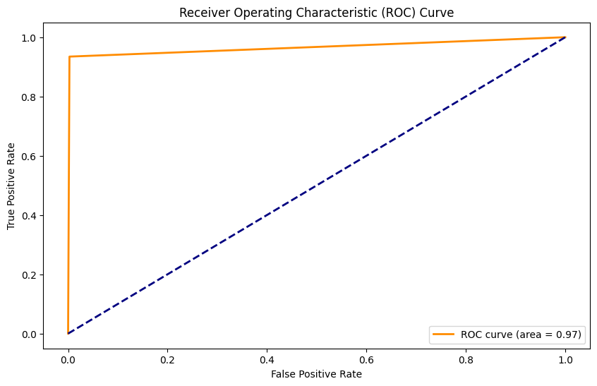
from sklearn.metrics import accuracy_score, precision_score, recall_score, f1_score, roc_curve, auc

y_pred = model.predict(X_test)
y_pred = (y_pred[:, 1] > 0.5).astype(int)

y_test = y_test[:, 1].astype(int)

# Calculate accuracy
accuracy = accuracy_score(y_test, y_pred)
print(f'Accuracy: {accuracy:.2f}')

# Calculate precision
precision = precision_score(y_test, y_pred)
print(f'Precision: {precision:.2f}')

# Calculate recall
recall = recall_score(y_test, y_pred)
print(f'Recall: {recall:.2f}')

# Calculate F1 Score
f1score = f1_score(y_test, y_pred)
print(f'F1 Score: {f1score:.2f}')

# Calculate ROC curve and AUC
fpr, tpr, thresholds = roc_curve(y_test, y_pred)
roc_auc = auc(fpr, tpr)

# Print AUC
print(f'AUC: {roc_auc:.2f}')

# Plot ROC curve
plt.figure(figsize=(10, 6))
plt.plot(fpr, tpr, color='darkorange', lw=2, label='ROC curve (area = {:.2f})'.format(roc_auc))
plt.plot([0, 1], [0, 1], color='navy', lw=2, linestyle='--')
plt.xlabel('False Positive Rate')
plt.ylabel('True Positive Rate')
plt.title('Receiver Operating Characteristic (ROC) Curve')
plt.legend(loc='lower right')
plt.show()
27/27 [==============================] - 1s 11ms/step
Accuracy: 0.99
Precision: 0.98
Recall: 0.93
F1 Score: 0.96
AUC: 0.97
LSTM con SMOTE#
# matriz de 9363 x 20
embedding_matrix = np.zeros((len(d2v_model.wv.index_to_key)+ 1, 20))

model_2 = Sequential()

model_2.add(Embedding(len(d2v_model.wv.index_to_key)+1,20,input_length=X.shape[1],weights=[embedding_matrix],trainable=True))

model_2.add(LSTM(50,return_sequences=False))

model_2.add(Dense(2,activation="softmax"))

model_2.compile(optimizer=Adam(),loss="binary_crossentropy",metrics = ['accuracy'])

batch_size = 32

history_2 = model_2.fit(X_train_smote, y_train_smote, epochs =50, batch_size=batch_size, verbose = 2)
Epoch 1/50
256/256 - 8s - loss: 0.3630 - accuracy: 0.8361 - 8s/epoch - 33ms/step
Epoch 2/50
256/256 - 6s - loss: 0.1362 - accuracy: 0.9559 - 6s/epoch - 23ms/step
Epoch 3/50
256/256 - 6s - loss: 0.0779 - accuracy: 0.9779 - 6s/epoch - 23ms/step
Epoch 4/50
256/256 - 6s - loss: 0.0452 - accuracy: 0.9878 - 6s/epoch - 23ms/step
Epoch 5/50
256/256 - 6s - loss: 0.0274 - accuracy: 0.9932 - 6s/epoch - 23ms/step
Epoch 6/50
256/256 - 6s - loss: 0.0188 - accuracy: 0.9951 - 6s/epoch - 22ms/step
Epoch 7/50
256/256 - 5s - loss: 0.0126 - accuracy: 0.9963 - 5s/epoch - 21ms/step
Epoch 8/50
256/256 - 5s - loss: 0.0063 - accuracy: 0.9982 - 5s/epoch - 21ms/step
Epoch 9/50
256/256 - 5s - loss: 0.0053 - accuracy: 0.9985 - 5s/epoch - 21ms/step
Epoch 10/50
256/256 - 5s - loss: 0.0033 - accuracy: 0.9990 - 5s/epoch - 21ms/step
Epoch 11/50
256/256 - 5s - loss: 0.0037 - accuracy: 0.9991 - 5s/epoch - 21ms/step
Epoch 12/50
256/256 - 5s - loss: 0.0043 - accuracy: 0.9989 - 5s/epoch - 21ms/step
Epoch 13/50
256/256 - 5s - loss: 0.0120 - accuracy: 0.9967 - 5s/epoch - 21ms/step
Epoch 14/50
256/256 - 5s - loss: 0.0035 - accuracy: 0.9988 - 5s/epoch - 21ms/step
Epoch 15/50
256/256 - 5s - loss: 0.0013 - accuracy: 0.9998 - 5s/epoch - 21ms/step
Epoch 16/50
256/256 - 5s - loss: 8.1742e-04 - accuracy: 0.9998 - 5s/epoch - 21ms/step
Epoch 17/50
256/256 - 5s - loss: 5.7329e-04 - accuracy: 0.9999 - 5s/epoch - 21ms/step
Epoch 18/50
256/256 - 5s - loss: 4.6134e-04 - accuracy: 0.9999 - 5s/epoch - 21ms/step
Epoch 19/50
256/256 - 5s - loss: 3.4523e-04 - accuracy: 1.0000 - 5s/epoch - 21ms/step
Epoch 20/50
256/256 - 5s - loss: 2.6883e-04 - accuracy: 0.9999 - 5s/epoch - 21ms/step
Epoch 21/50
256/256 - 5s - loss: 2.2418e-04 - accuracy: 1.0000 - 5s/epoch - 21ms/step
Epoch 22/50
256/256 - 5s - loss: 1.5771e-04 - accuracy: 1.0000 - 5s/epoch - 21ms/step
Epoch 23/50
256/256 - 5s - loss: 1.3357e-04 - accuracy: 1.0000 - 5s/epoch - 21ms/step
Epoch 24/50
256/256 - 5s - loss: 1.1690e-04 - accuracy: 1.0000 - 5s/epoch - 21ms/step
Epoch 25/50
256/256 - 5s - loss: 7.7140e-05 - accuracy: 1.0000 - 5s/epoch - 21ms/step
Epoch 26/50
256/256 - 5s - loss: 6.9837e-05 - accuracy: 1.0000 - 5s/epoch - 21ms/step
Epoch 27/50
256/256 - 5s - loss: 5.4699e-05 - accuracy: 1.0000 - 5s/epoch - 21ms/step
Epoch 28/50
256/256 - 5s - loss: 4.6409e-05 - accuracy: 1.0000 - 5s/epoch - 21ms/step
Epoch 29/50
256/256 - 5s - loss: 4.0961e-05 - accuracy: 1.0000 - 5s/epoch - 21ms/step
Epoch 30/50
256/256 - 6s - loss: 3.0426e-05 - accuracy: 1.0000 - 6s/epoch - 22ms/step
Epoch 31/50
256/256 - 6s - loss: 2.4787e-05 - accuracy: 1.0000 - 6s/epoch - 23ms/step
Epoch 32/50
256/256 - 6s - loss: 2.0901e-05 - accuracy: 1.0000 - 6s/epoch - 22ms/step
Epoch 33/50
256/256 - 6s - loss: 1.6103e-05 - accuracy: 1.0000 - 6s/epoch - 23ms/step
Epoch 34/50
256/256 - 6s - loss: 1.4357e-05 - accuracy: 1.0000 - 6s/epoch - 22ms/step
Epoch 35/50
256/256 - 6s - loss: 1.2146e-05 - accuracy: 1.0000 - 6s/epoch - 22ms/step
Epoch 36/50
256/256 - 5s - loss: 1.0225e-05 - accuracy: 1.0000 - 5s/epoch - 20ms/step
Epoch 37/50
256/256 - 5s - loss: 8.4397e-06 - accuracy: 1.0000 - 5s/epoch - 20ms/step
Epoch 38/50
256/256 - 5s - loss: 7.2955e-06 - accuracy: 1.0000 - 5s/epoch - 20ms/step
Epoch 39/50
256/256 - 5s - loss: 6.3138e-06 - accuracy: 1.0000 - 5s/epoch - 20ms/step
Epoch 40/50
256/256 - 5s - loss: 5.3885e-06 - accuracy: 1.0000 - 5s/epoch - 20ms/step
Epoch 41/50
256/256 - 5s - loss: 4.5613e-06 - accuracy: 1.0000 - 5s/epoch - 20ms/step
Epoch 42/50
256/256 - 5s - loss: 3.9344e-06 - accuracy: 1.0000 - 5s/epoch - 20ms/step
Epoch 43/50
256/256 - 5s - loss: 3.3964e-06 - accuracy: 1.0000 - 5s/epoch - 20ms/step
Epoch 44/50
256/256 - 5s - loss: 2.8711e-06 - accuracy: 1.0000 - 5s/epoch - 20ms/step
Epoch 45/50
256/256 - 5s - loss: 2.4272e-06 - accuracy: 1.0000 - 5s/epoch - 20ms/step
Epoch 46/50
256/256 - 5s - loss: 2.1240e-06 - accuracy: 1.0000 - 5s/epoch - 20ms/step
Epoch 47/50
256/256 - 5s - loss: 1.8127e-06 - accuracy: 1.0000 - 5s/epoch - 20ms/step
Epoch 48/50
256/256 - 5s - loss: 1.6042e-06 - accuracy: 1.0000 - 5s/epoch - 21ms/step
Epoch 49/50
256/256 - 5s - loss: 1.3917e-06 - accuracy: 1.0000 - 5s/epoch - 20ms/step
Epoch 50/50
256/256 - 5s - loss: 1.1890e-06 - accuracy: 1.0000 - 5s/epoch - 21ms/step
y_pred = model_2.predict(X_test)
y_pred = (y_pred[:, 1] > 0.5).astype(int)

# Calculate accuracy
accuracy = accuracy_score(y_test, y_pred)
print(f'Accuracy: {accuracy:.2f}')

# Calculate precision
precision = precision_score(y_test, y_pred)
print(f'Precision: {precision:.2f}')

# Calculate recall
recall = recall_score(y_test, y_pred)
print(f'Recall: {recall:.2f}')

# Calculate F1 Score
f1score = f1_score(y_test, y_pred)
print(f'F1 Score: {f1score:.2f}')

# Calculate ROC curve and AUC
fpr, tpr, thresholds = roc_curve(y_test, y_pred)
roc_auc = auc(fpr, tpr)

# Print AUC
print(f'AUC: {roc_auc:.2f}')

# Plot ROC curve
plt.figure(figsize=(10, 6))
plt.plot(fpr, tpr, color='darkorange', lw=2, label='ROC curve (area = {:.2f})'.format(roc_auc))
plt.plot([0, 1], [0, 1], color='navy', lw=2, linestyle='--')
plt.xlabel('False Positive Rate')
plt.ylabel('True Positive Rate')
plt.title('Receiver Operating Characteristic (ROC) Curve')
plt.legend(loc='lower right')
plt.show()
27/27 [==============================] - 1s 11ms/step
Accuracy: 0.91
Precision: 0.58
Recall: 0.95
F1 Score: 0.72
AUC: 0.93

KNN#
from sklearn.model_selection import GridSearchCV
from sklearn.neighbors import KNeighborsClassifier
from sklearn.metrics import make_scorer, f1_score

# Define the kNN classifier
knn_classifier = KNeighborsClassifier()

# Define the hyperparameters and their possible values
param_grid = {'n_neighbors': [3, 5, 7], 'weights': ['uniform', 'distance']}

# Create a F1 scorer for grid search
f1_scorer = make_scorer(f1_score)

# Create GridSearchCV object
grid_search = GridSearchCV(knn_classifier, param_grid, scoring=f1_scorer, cv=5)

# Fit the grid search to the data
grid_search.fit(X_train, y_train)

# Print the best hyperparameters
print("Best Hyperparameters:", grid_search.best_params_)

# Get the best model
best_knn_model = grid_search.best_estimator_

# Make predictions on the test set
y_pred = best_knn_model.predict(X_test)
y_pred = (y_pred[:, 1] > 0.5).astype(int)

# Calculate F1 Score on the test set
f1score = f1_score(y_test, y_pred)
print(f'F1 Score on Test Set: {f1score:.2f}')
Best Hyperparameters: {'n_neighbors': 3, 'weights': 'uniform'}
F1 Score on Test Set: 0.48
from sklearn.neighbors import KNeighborsClassifier

# Create a kNN classifier
knn_classifier = KNeighborsClassifier(n_neighbors=3, weights='uniform')

# Train the classifier on the training data
knn_classifier.fit(X_train, y_train)

# Make predictions on the testing data
y_pred = knn_classifier.predict(X_test)
y_pred = (y_pred[:, 1] > 0.5).astype(int)
# Calculate accuracy
accuracy = accuracy_score(y_test, y_pred)
print(f'Accuracy: {accuracy:.2f}')

# Calculate precision
precision = precision_score(y_test, y_pred)
print(f'Precision: {precision:.2f}')

# Calculate recall
recall = recall_score(y_test, y_pred)
print(f'Recall: {recall:.2f}')

# Calculate F1 Score
f1score = f1_score(y_test, y_pred)
print(f'F1 Score: {f1score:.2f}')

# Calculate ROC curve and AUC
fpr, tpr, thresholds = roc_curve(y_test, y_pred)
roc_auc = auc(fpr, tpr)

# Print AUC
print(f'AUC: {roc_auc:.2f}')

# Plot ROC curve
plt.figure(figsize=(10, 6))
plt.plot(fpr, tpr, color='darkorange', lw=2, label='ROC curve (area = {:.2f})'.format(roc_auc))
plt.plot([0, 1], [0, 1], color='navy', lw=2, linestyle='--')
plt.xlabel('False Positive Rate')
plt.ylabel('True Positive Rate')
plt.title('Receiver Operating Characteristic (ROC) Curve')
plt.legend(loc='lower right')
plt.show()
Accuracy: 0.88
Precision: 0.55
Recall: 0.43
F1 Score: 0.48
AUC: 0.69
KNN con SMOTE#
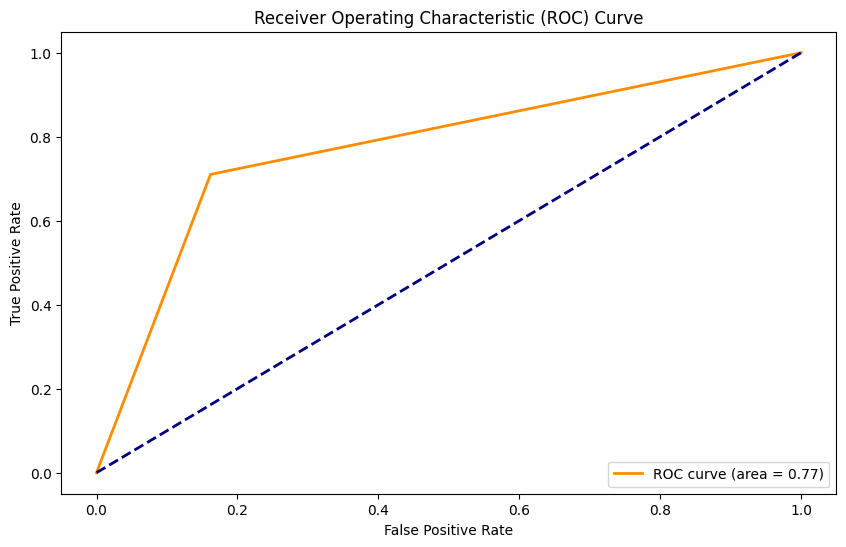
# Create a kNN classifier
knn_classifier = KNeighborsClassifier(n_neighbors=3, weights='uniform')

# Train the classifier on the training data
knn_classifier.fit(X_train_smote, y_train_smote)

# Make predictions on the testing data
y_pred = knn_classifier.predict(X_test)
y_pred = (y_pred[:, 1] > 0.5).astype(int)
# Calculate accuracy
accuracy = accuracy_score(y_test, y_pred)
print(f'Accuracy: {accuracy:.2f}')

# Calculate precision
precision = precision_score(y_test, y_pred)
print(f'Precision: {precision:.2f}')

# Calculate recall
recall = recall_score(y_test, y_pred)
print(f'Recall: {recall:.2f}')

# Calculate F1 Score
f1score = f1_score(y_test, y_pred)
print(f'F1 Score: {f1score:.2f}')

# Calculate ROC curve and AUC
fpr, tpr, thresholds = roc_curve(y_test, y_pred)
roc_auc = auc(fpr, tpr)

# Print AUC
print(f'AUC: {roc_auc:.2f}')

# Plot ROC curve
plt.figure(figsize=(10, 6))
plt.plot(fpr, tpr, color='darkorange', lw=2, label='ROC curve (area = {:.2f})'.format(roc_auc))
plt.plot([0, 1], [0, 1], color='navy', lw=2, linestyle='--')
plt.xlabel('False Positive Rate')
plt.ylabel('True Positive Rate')
plt.title('Receiver Operating Characteristic (ROC) Curve')
plt.legend(loc='lower right')
plt.show()
Accuracy: 0.82
Precision: 0.39
Recall: 0.71
F1 Score: 0.50
AUC: 0.77
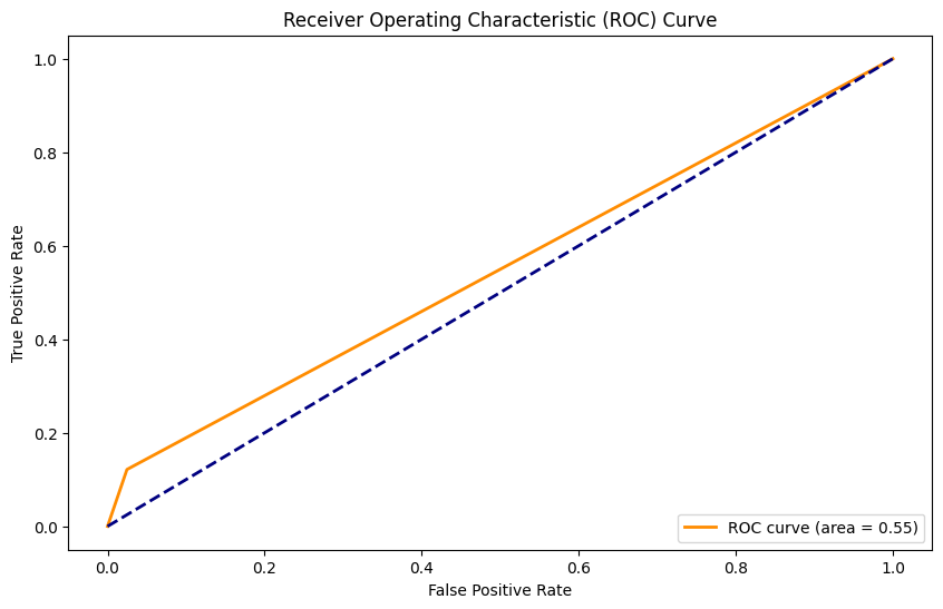
Ridge Classifier#
from sklearn.model_selection import GridSearchCV
from sklearn.linear_model import RidgeClassifier
from sklearn.metrics import make_scorer, f1_score

# Define the Ridge classifier
ridge_classifier = RidgeClassifier()

# Define the hyperparameters and their possible values
param_grid = {'alpha': [0.1, 1.0, 10.0], 'solver': ['auto', 'svd', 'cholesky', 'lsqr', 'sparse_cg', 'sag', 'saga']}

# Create a F1 scorer for grid search
f1_scorer = make_scorer(f1_score)

# Create GridSearchCV object
grid_search = GridSearchCV(ridge_classifier, param_grid, scoring=f1_scorer, cv=5)

# Fit the grid search to the data
grid_search.fit(X_train, y_train)

# Print the best hyperparameters
print("Best Hyperparameters:", grid_search.best_params_)

# Get the best model
best_ridge_model = grid_search.best_estimator_

# Make predictions on the test set
y_pred = best_ridge_model.predict(X_test)
y_pred = (y_pred[:, 1] > 0.5).astype(int)

# Calculate F1 Score on the test set
f1score = f1_score(y_test, y_pred)
print(f'F1 Score on Test Set: {f1score:.2f}')
Best Hyperparameters: {'alpha': 0.1, 'solver': 'auto'}
F1 Score on Test Set: 0.19
ridge_classifier = RidgeClassifier(alpha = 0.1, solver = 'auto')

# Train the classifier on the training data
ridge_classifier.fit(X_train, y_train)

# Make predictions on the testing data
y_pred = ridge_classifier.predict(X_test)
y_pred = (y_pred[:, 1] > 0.5).astype(int)

# Calculate accuracy
accuracy = accuracy_score(y_test, y_pred)
print(f'Accuracy: {accuracy:.2f}')

# Calculate precision
precision = precision_score(y_test, y_pred)
print(f'Precision: {precision:.2f}')

# Calculate recall
recall = recall_score(y_test, y_pred)
print(f'Recall: {recall:.2f}')

# Calculate F1 Score
f1score = f1_score(y_test, y_pred)
print(f'F1 Score: {f1score:.2f}')

# Calculate ROC curve and AUC
fpr, tpr, thresholds = roc_curve(y_test, y_pred)
roc_auc = auc(fpr, tpr)

# Print AUC
print(f'AUC: {roc_auc:.2f}')

# Plot ROC curve
plt.figure(figsize=(10, 6))
plt.plot(fpr, tpr, color='darkorange', lw=2, label='ROC curve (area = {:.2f})'.format(roc_auc))
plt.plot([0, 1], [0, 1], color='navy', lw=2, linestyle='--')
plt.xlabel('False Positive Rate')
plt.ylabel('True Positive Rate')
plt.title('Receiver Operating Characteristic (ROC) Curve')
plt.legend(loc='lower right')
plt.show()
Accuracy: 0.87
Precision: 0.42
Recall: 0.12
F1 Score: 0.19
AUC: 0.55
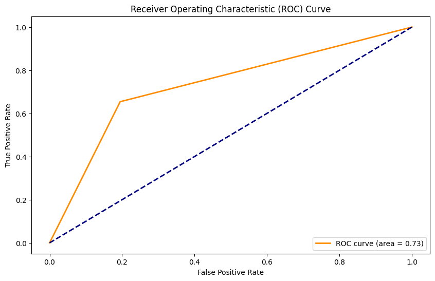
Ridge Classifier con SMOTE#
ridge_classifier = RidgeClassifier(alpha = 0.1, solver = 'auto')

# Train the classifier on the training data
ridge_classifier.fit(X_train_smote, y_train_smote)

# Make predictions on the testing data
y_pred = ridge_classifier.predict(X_test)
y_pred = (y_pred[:, 1] > 0.5).astype(int)

# Calculate accuracy
accuracy = accuracy_score(y_test, y_pred)
print(f'Accuracy: {accuracy:.2f}')

# Calculate precision
precision = precision_score(y_test, y_pred)
print(f'Precision: {precision:.2f}')

# Calculate recall
recall = recall_score(y_test, y_pred)
print(f'Recall: {recall:.2f}')

# Calculate F1 Score
f1score = f1_score(y_test, y_pred)
print(f'F1 Score: {f1score:.2f}')

# Calculate ROC curve and AUC
fpr, tpr, thresholds = roc_curve(y_test, y_pred)
roc_auc = auc(fpr, tpr)

# Print AUC
print(f'AUC: {roc_auc:.2f}')

# Plot ROC curve
plt.figure(figsize=(10, 6))
plt.plot(fpr, tpr, color='darkorange', lw=2, label='ROC curve (area = {:.2f})'.format(roc_auc))
plt.plot([0, 1], [0, 1], color='navy', lw=2, linestyle='--')
plt.xlabel('False Positive Rate')
plt.ylabel('True Positive Rate')
plt.title('Receiver Operating Characteristic (ROC) Curve')
plt.legend(loc='lower right')
plt.show()
Accuracy: 0.78
Precision: 0.33
Recall: 0.65
F1 Score: 0.44
AUC: 0.73

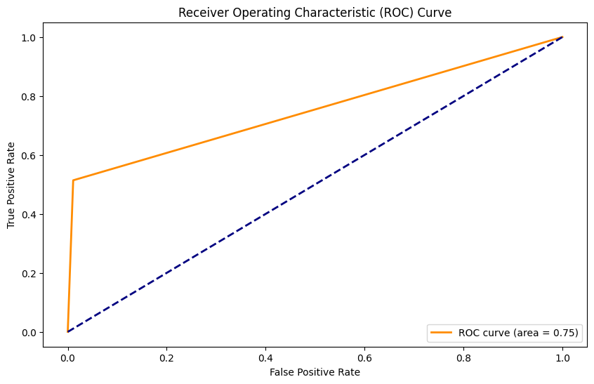
Naive Bayes Classifier#
from sklearn.naive_bayes import MultinomialNB

# Define the Naive Bayes model
naive_bayes = MultinomialNB()

# Define the parameter grid to search
param_grid = {
    'alpha': np.linspace(0.1, 1.0, 10),  # Adjust as needed
    'fit_prior': [True, False]
}

# Create F1 scorer
f1_scorer = make_scorer(f1_score)

# Initialize GridSearchCV
grid_search = GridSearchCV(naive_bayes, param_grid, cv=5, scoring=f1_scorer)

# Fit the grid search to the data
grid_search.fit(X_train, y_train[:, 1].astype(int))

# Print the best parameters and corresponding F1 score
print("Best Hyperparameters:", grid_search.best_params_)
print("Best F1 Score:", grid_search.best_score_)
Best Hyperparameters: {'alpha': 0.1, 'fit_prior': True}
Best F1 Score: 0.43899155529615747
# Create a kNN classifier with k=3
naive_bayes = MultinomialNB(alpha=0.1, fit_prior=True)

# Train the classifier on the training data
naive_bayes.fit(X_train, y_train[:, 1].astype(int))

# Make predictions on the testing data
y_pred = naive_bayes.predict(X_test)

# Calculate accuracy
accuracy = accuracy_score(y_test, y_pred)
print(f'Accuracy: {accuracy:.2f}')

# Calculate precision
precision = precision_score(y_test, y_pred)
print(f'Precision: {precision:.2f}')

# Calculate recall
recall = recall_score(y_test, y_pred)
print(f'Recall: {recall:.2f}')

# Calculate F1 Score
f1score = f1_score(y_test, y_pred)
print(f'F1 Score: {f1score:.2f}')

# Calculate ROC curve and AUC
fpr, tpr, thresholds = roc_curve(y_test, y_pred)
roc_auc = auc(fpr, tpr)

# Print AUC
print(f'AUC: {roc_auc:.2f}')

# Plot ROC curve
plt.figure(figsize=(10, 6))
plt.plot(fpr, tpr, color='darkorange', lw=2, label='ROC curve (area = {:.2f})'.format(roc_auc))
plt.plot([0, 1], [0, 1], color='navy', lw=2, linestyle='--')
plt.xlabel('False Positive Rate')
plt.ylabel('True Positive Rate')
plt.title('Receiver Operating Characteristic (ROC) Curve')
plt.legend(loc='lower right')
plt.show()
Accuracy: 0.79
Precision: 0.33
Recall: 0.65
F1 Score: 0.44
AUC: 0.73
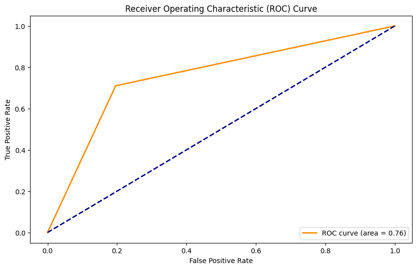
Naiva Bayes Classifier con SMOTE#
# Create a kNN classifier with k=3
naive_bayes = MultinomialNB(alpha=0.1, fit_prior=True)

# Train the classifier on the training data
naive_bayes.fit(X_train_smote, y_train_smote[:, 1].astype(int))

# Make predictions on the testing data
y_pred = naive_bayes.predict(X_test)

# Calculate accuracy
accuracy = accuracy_score(y_test, y_pred)
print(f'Accuracy: {accuracy:.2f}')

# Calculate precision
precision = precision_score(y_test, y_pred)
print(f'Precision: {precision:.2f}')

# Calculate recall
recall = recall_score(y_test, y_pred)
print(f'Recall: {recall:.2f}')

# Calculate F1 Score
f1score = f1_score(y_test, y_pred)
print(f'F1 Score: {f1score:.2f}')

# Calculate ROC curve and AUC
fpr, tpr, thresholds = roc_curve(y_test, y_pred)
roc_auc = auc(fpr, tpr)

# Print AUC
print(f'AUC: {roc_auc:.2f}')

# Plot ROC curve
plt.figure(figsize=(10, 6))
plt.plot(fpr, tpr, color='darkorange', lw=2, label='ROC curve (area = {:.2f})'.format(roc_auc))
plt.plot([0, 1], [0, 1], color='navy', lw=2, linestyle='--')
plt.xlabel('False Positive Rate')
plt.ylabel('True Positive Rate')
plt.title('Receiver Operating Characteristic (ROC) Curve')
plt.legend(loc='lower right')
plt.show()
Accuracy: 0.79
Precision: 0.35
Recall: 0.71
F1 Score: 0.47
AUC: 0.76
Random Forest Classifier#
from sklearn.model_selection import GridSearchCV
from sklearn.ensemble import RandomForestClassifier
from sklearn.metrics import make_scorer, f1_score

# Define the Random Forest model
rf_model = RandomForestClassifier()

param_grid = {
    'n_estimators': [50, 100, 200],
    'max_depth': [3, 5, 7],
    'min_samples_split': [2, 5, 10],
    'min_samples_leaf': [1, 2, 4],
    'class_weight': [None, 'balanced', 'balanced_subsample']
}

# Create F1 scorer
f1_scorer = make_scorer(f1_score)

# Initialize GridSearchCV
grid_search = GridSearchCV(rf_model, param_grid, cv=5, scoring=f1_scorer)

# Fit the grid search to the data
grid_search.fit(X_train, y_train[:, 1].astype(int))

# Print the best parameters and corresponding F1 score
print("Best Hyperparameters:", grid_search.best_params_)
print("Best F1 Score:", grid_search.best_score_)
Best Hyperparameters: {'class_weight': None, 'max_depth': 7, 'min_samples_leaf': 1, 'min_samples_split': 5, 'n_estimators': 200}
Best F1 Score: 0.6555674195944813
from sklearn.metrics import accuracy_score, precision_score, recall_score, f1_score, roc_curve, auc
from sklearn.ensemble import RandomForestClassifier
import matplotlib.pyplot as plt

rf_model = RandomForestClassifier(n_estimators=200,
                                  max_depth=7,
                                  min_samples_leaf = 1,
                                  min_samples_split = 5,
                                  class_weight = None)

# Train the classifier on the training data
rf_model.fit(X_train, y_train[:, 1].astype(int))

# Make predictions on the testing data
y_pred_rf = rf_model.predict(X_test)

# Get unique values in the array
unique_values = np.unique(y_pred_rf)
# Initialize one-hot encoded array with zeros
y_pred = np.zeros((len(y_pred_rf), len(unique_values)))
# Fill in the one-hot array based on the original binary array
for i, value in enumerate(y_pred_rf):
    y_pred[i, np.where(unique_values == value)] = 1

# Calculate accuracy
accuracy = accuracy_score(y_test[:, 1].astype(int), np.argmax(y_pred, axis=1))
print(f'Accuracy: {accuracy:.2f}')

# Calculate precision
precision = precision_score(y_test[:, 1].astype(int), np.argmax(y_pred, axis=1))
print(f'Precision: {precision:.2f}')

# Calculate recall
recall = recall_score(y_test[:, 1].astype(int), np.argmax(y_pred, axis=1))
print(f'Recall: {recall:.2f}')

# Calculate F1 Score
f1score = f1_score(y_test[:, 1].astype(int), np.argmax(y_pred, axis=1))
print(f'F1 Score: {f1score:.2f}')

# Calculate ROC curve and AUC
fpr, tpr, thresholds = roc_curve(y_test[:, 1].astype(int), np.argmax(y_pred, axis=1))
roc_auc = auc(fpr, tpr)

# Print AUC
print(f'AUC: {roc_auc:.2f}')

# Plot ROC curve
plt.figure(figsize=(10, 6))
plt.plot(fpr, tpr, color='darkorange', lw=2, label='ROC curve (area = {:.2f})'.format(roc_auc))
plt.plot([0, 1], [0, 1], color='navy', lw=2, linestyle='--')
plt.xlabel('False Positive Rate')
plt.ylabel('True Positive Rate')
plt.title('Receiver Operating Characteristic (ROC) Curve')
plt.legend(loc='lower right')
plt.show()
Accuracy: 0.93
Precision: 0.87
Recall: 0.51
F1 Score: 0.65
AUC: 0.75
Random Forest Classifier con SMOTE#
from sklearn.metrics import accuracy_score, precision_score, recall_score, f1_score, roc_curve, auc
from sklearn.ensemble import RandomForestClassifier
import matplotlib.pyplot as plt

rf_model = RandomForestClassifier(n_estimators=200,
                                  max_depth=7,
                                  min_samples_leaf = 1,
                                  min_samples_split = 5,
                                  class_weight = None)

# Train the classifier on the training data
rf_model.fit(X_train_smote, y_train_smote[:, 1].astype(int))

# Make predictions on the testing data
y_pred_rf = rf_model.predict(X_test)

# Get unique values in the array
unique_values = np.unique(y_pred_rf)
# Initialize one-hot encoded array with zeros
y_pred = np.zeros((len(y_pred_rf), len(unique_values)))
# Fill in the one-hot array based on the original binary array
for i, value in enumerate(y_pred_rf):
    y_pred[i, np.where(unique_values == value)] = 1

# Calculate accuracy
accuracy = accuracy_score(y_test[:, 1].astype(int), np.argmax(y_pred, axis=1))
print(f'Accuracy: {accuracy:.2f}')

# Calculate precision
precision = precision_score(y_test[:, 1].astype(int), np.argmax(y_pred, axis=1))
print(f'Precision: {precision:.2f}')

# Calculate recall
recall = recall_score(y_test[:, 1].astype(int), np.argmax(y_pred, axis=1))
print(f'Recall: {recall:.2f}')

# Calculate F1 Score
f1score = f1_score(y_test[:, 1].astype(int), np.argmax(y_pred, axis=1))
print(f'F1 Score: {f1score:.2f}')

# Calculate ROC curve and AUC
fpr, tpr, thresholds = roc_curve(y_test[:, 1].astype(int), np.argmax(y_pred, axis=1))
roc_auc = auc(fpr, tpr)

# Print AUC
print(f'AUC: {roc_auc:.2f}')

# Plot ROC curve
plt.figure(figsize=(10, 6))
plt.plot(fpr, tpr, color='darkorange', lw=2, label='ROC curve (area = {:.2f})'.format(roc_auc))
plt.plot([0, 1], [0, 1], color='navy', lw=2, linestyle='--')
plt.xlabel('False Positive Rate')
plt.ylabel('True Positive Rate')
plt.title('Receiver Operating Characteristic (ROC) Curve')
plt.legend(loc='lower right')
plt.show()
Accuracy: 0.86
Precision: 0.48
Recall: 0.80
F1 Score: 0.60
AUC: 0.84
Nueva propuesta: Stacked model#
from sklearn.linear_model import LogisticRegression
from keras.models import Sequential
from keras.layers import LSTM, Dense, Embedding
from tensorflow.keras.optimizers.legacy import Adam
from sklearn.neighbors import KNeighborsClassifier

X_trainval, X_test, y_trainval, y_test = train_test_split(X, Y, test_size = 0.15, random_state = 42)

X_train, X_valid, y_train, y_valid = train_test_split(X_trainval, y_trainval, test_size=0.2, random_state=42)

################## LSTM ##################

# matriz de 9363 x 20
embedding_matrix = np.zeros((len(d2v_model.wv.index_to_key)+ 1, 20))

model = Sequential()

model.add(Embedding(len(d2v_model.wv.index_to_key)+1,20,input_length=X.shape[1],weights=[embedding_matrix],trainable=True))

model.add(LSTM(50,return_sequences=False))

model.add(Dense(2,activation="softmax"))

model.compile(optimizer=Adam(),loss="binary_crossentropy",metrics = ['accuracy'])

batch_size = 32

history = model.fit(X_train, y_train, epochs =50, batch_size=batch_size, verbose = 2)

################## KNN ############################

# Create a kNN classifier
knn_classifier = KNeighborsClassifier(n_neighbors=3, weights='uniform')

# Train the classifier on the training data
knn_classifier.fit(X_train, y_train)
Epoch 1/50
119/119 - 6s - loss: 0.3772 - accuracy: 0.8738 - 6s/epoch - 49ms/step
Epoch 2/50
119/119 - 3s - loss: 0.0801 - accuracy: 0.9810 - 3s/epoch - 27ms/step
Epoch 3/50
119/119 - 3s - loss: 0.0316 - accuracy: 0.9916 - 3s/epoch - 27ms/step
Epoch 4/50
119/119 - 3s - loss: 0.0154 - accuracy: 0.9968 - 3s/epoch - 27ms/step
Epoch 5/50
119/119 - 3s - loss: 0.0098 - accuracy: 0.9974 - 3s/epoch - 26ms/step
Epoch 6/50
119/119 - 3s - loss: 0.0054 - accuracy: 0.9987 - 3s/epoch - 25ms/step
Epoch 7/50
119/119 - 3s - loss: 0.0042 - accuracy: 0.9989 - 3s/epoch - 25ms/step
Epoch 8/50
119/119 - 3s - loss: 0.0041 - accuracy: 0.9992 - 3s/epoch - 25ms/step
Epoch 9/50
119/119 - 3s - loss: 0.0028 - accuracy: 0.9995 - 3s/epoch - 23ms/step
Epoch 10/50
119/119 - 3s - loss: 0.0013 - accuracy: 0.9997 - 3s/epoch - 23ms/step
Epoch 11/50
119/119 - 3s - loss: 0.0014 - accuracy: 0.9997 - 3s/epoch - 23ms/step
Epoch 12/50
119/119 - 3s - loss: 9.4009e-04 - accuracy: 0.9997 - 3s/epoch - 23ms/step
Epoch 13/50
119/119 - 3s - loss: 7.3789e-04 - accuracy: 0.9997 - 3s/epoch - 23ms/step
Epoch 14/50
119/119 - 3s - loss: 5.4639e-04 - accuracy: 0.9997 - 3s/epoch - 23ms/step
Epoch 15/50
119/119 - 3s - loss: 6.1255e-04 - accuracy: 0.9997 - 3s/epoch - 24ms/step
Epoch 16/50
119/119 - 3s - loss: 3.8961e-04 - accuracy: 1.0000 - 3s/epoch - 23ms/step
Epoch 17/50
119/119 - 3s - loss: 3.0204e-04 - accuracy: 1.0000 - 3s/epoch - 23ms/step
Epoch 18/50
119/119 - 3s - loss: 2.7991e-04 - accuracy: 1.0000 - 3s/epoch - 25ms/step
Epoch 19/50
119/119 - 3s - loss: 2.7193e-04 - accuracy: 1.0000 - 3s/epoch - 25ms/step
Epoch 20/50
119/119 - 3s - loss: 1.9108e-04 - accuracy: 1.0000 - 3s/epoch - 23ms/step
Epoch 21/50
119/119 - 3s - loss: 1.7832e-04 - accuracy: 1.0000 - 3s/epoch - 24ms/step
Epoch 22/50
119/119 - 3s - loss: 1.3178e-04 - accuracy: 1.0000 - 3s/epoch - 24ms/step
Epoch 23/50
119/119 - 3s - loss: 1.1231e-04 - accuracy: 1.0000 - 3s/epoch - 26ms/step
Epoch 24/50
119/119 - 3s - loss: 1.0353e-04 - accuracy: 1.0000 - 3s/epoch - 28ms/step
Epoch 25/50
119/119 - 3s - loss: 9.9223e-05 - accuracy: 1.0000 - 3s/epoch - 27ms/step
Epoch 26/50
119/119 - 3s - loss: 7.6312e-05 - accuracy: 1.0000 - 3s/epoch - 26ms/step
Epoch 27/50
119/119 - 3s - loss: 6.6245e-05 - accuracy: 1.0000 - 3s/epoch - 26ms/step
Epoch 28/50
119/119 - 3s - loss: 6.7231e-05 - accuracy: 1.0000 - 3s/epoch - 27ms/step
Epoch 29/50
119/119 - 3s - loss: 4.9366e-05 - accuracy: 1.0000 - 3s/epoch - 25ms/step
Epoch 30/50
119/119 - 3s - loss: 4.4229e-05 - accuracy: 1.0000 - 3s/epoch - 27ms/step
Epoch 31/50
119/119 - 3s - loss: 3.8014e-05 - accuracy: 1.0000 - 3s/epoch - 26ms/step
Epoch 32/50
119/119 - 3s - loss: 3.3968e-05 - accuracy: 1.0000 - 3s/epoch - 26ms/step
Epoch 33/50
119/119 - 3s - loss: 4.0132e-05 - accuracy: 1.0000 - 3s/epoch - 25ms/step
Epoch 34/50
119/119 - 3s - loss: 0.0569 - accuracy: 0.9926 - 3s/epoch - 26ms/step
Epoch 35/50
119/119 - 3s - loss: 0.0075 - accuracy: 0.9974 - 3s/epoch - 28ms/step
Epoch 36/50
119/119 - 3s - loss: 0.0020 - accuracy: 0.9995 - 3s/epoch - 24ms/step
Epoch 37/50
119/119 - 3s - loss: 0.0022 - accuracy: 0.9995 - 3s/epoch - 24ms/step
Epoch 38/50
119/119 - 3s - loss: 9.3576e-04 - accuracy: 0.9997 - 3s/epoch - 28ms/step
Epoch 39/50
119/119 - 3s - loss: 6.2406e-04 - accuracy: 0.9997 - 3s/epoch - 29ms/step
Epoch 40/50
119/119 - 3s - loss: 5.0593e-04 - accuracy: 1.0000 - 3s/epoch - 26ms/step
Epoch 41/50
119/119 - 3s - loss: 4.2122e-04 - accuracy: 1.0000 - 3s/epoch - 24ms/step
Epoch 42/50
119/119 - 3s - loss: 3.5127e-04 - accuracy: 1.0000 - 3s/epoch - 26ms/step
Epoch 43/50
119/119 - 3s - loss: 2.9751e-04 - accuracy: 1.0000 - 3s/epoch - 27ms/step
Epoch 44/50
119/119 - 3s - loss: 2.5839e-04 - accuracy: 1.0000 - 3s/epoch - 26ms/step
Epoch 45/50
119/119 - 3s - loss: 2.2521e-04 - accuracy: 1.0000 - 3s/epoch - 24ms/step
Epoch 46/50
119/119 - 3s - loss: 1.9927e-04 - accuracy: 1.0000 - 3s/epoch - 28ms/step
Epoch 47/50
119/119 - 4s - loss: 1.7689e-04 - accuracy: 1.0000 - 4s/epoch - 30ms/step
Epoch 48/50
119/119 - 3s - loss: 1.5731e-04 - accuracy: 1.0000 - 3s/epoch - 26ms/step
Epoch 49/50
119/119 - 3s - loss: 1.4191e-04 - accuracy: 1.0000 - 3s/epoch - 25ms/step
Epoch 50/50
119/119 - 3s - loss: 1.2780e-04 - accuracy: 1.0000 - 3s/epoch - 25ms/step
KNeighborsClassifier(n_neighbors=3)In a Jupyter environment, please rerun this cell to show the HTML representation or trust the notebook.
On GitHub, the HTML representation is unable to render, please try loading this page with nbviewer.org.
KNeighborsClassifier(n_neighbors=3)
from sklearn.linear_model import LogisticRegression

# Hacer predicciones en el conjunto de validación
pred1 = model.predict(X_valid)

pred2 = knn_classifier.predict(X_valid)

# Stack predicciones para crear nuevas características para el meta-modelo
stacked_predictions = np.column_stack((pred1, pred2))

# Entrenar el meta-modelo
meta_model = LogisticRegression()

y_valid_onehot = y_valid[:, 1].astype(int)

meta_model.fit(stacked_predictions, y_valid_onehot)

# Para hacer predicciones en nuevos datos
new_pred1 = model.predict(X_test)

new_pred2 = knn_classifier.predict(X_test)

stacked_new_predictions = np.column_stack((new_pred1, new_pred2))

final_predictions = meta_model.predict(stacked_new_predictions)
30/30 [==============================] - 1s 11ms/step
27/27 [==============================] - 0s 10ms/step
from sklearn.metrics import accuracy_score, classification_report, confusion_matrix
import seaborn as sns
import matplotlib.pyplot as plt

# Calcular y mostrar la precisión
Y_test_onehot = y_test[:, 1].astype(int)

# Calculate accuracy
accuracy = accuracy_score(Y_test_onehot, final_predictions)
print(f'Accuracy: {accuracy:.2f}')

# Calculate precision
precision = precision_score(Y_test_onehot, final_predictions)
print(f'Precision: {precision:.2f}')

# Calculate recall
recall = recall_score(Y_test_onehot, final_predictions)
print(f'Recall: {recall:.2f}')

# Calculate F1 Score
f1score = f1_score(Y_test_onehot, final_predictions)
print(f'F1 Score: {f1score:.2f}')

# Calculate ROC curve and AUC
fpr, tpr, thresholds = roc_curve(Y_test_onehot, final_predictions)
roc_auc = auc(fpr, tpr)

# Print AUC
print(f'AUC: {roc_auc:.2f}')

# Plot ROC curve
plt.figure(figsize=(10, 6))
plt.plot(fpr, tpr, color='darkorange', lw=2, label='ROC curve (area = {:.2f})'.format(roc_auc))
plt.plot([0, 1], [0, 1], color='navy', lw=2, linestyle='--')
plt.xlabel('False Positive Rate')
plt.ylabel('True Positive Rate')
plt.title('Receiver Operating Characteristic (ROC) Curve')
plt.legend(loc='lower right')
plt.show()
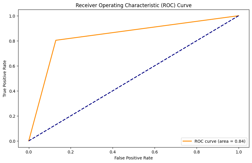
Accuracy: 0.99
Precision: 0.98
Recall: 0.93
F1 Score: 0.95
AUC: 0.96
Stacked Model con SMOTE#
from sklearn.linear_model import LogisticRegression
from keras.models import Sequential
from keras.layers import LSTM, Dense, Embedding
from tensorflow.keras.optimizers.legacy import Adam
from sklearn.neighbors import KNeighborsClassifier

X_trainval, X_test, y_trainval, y_test = train_test_split(X, Y, test_size = 0.15, random_state = 42)

X_train, X_valid, y_train, y_valid = train_test_split(X_trainval, y_trainval, test_size=0.2, random_state=42)

################## SMOTE #################

from imblearn.over_sampling import SMOTE

# Crear una instancia de SMOTE
smote = SMOTE(random_state=42)

y_for_smote = np.argmax(y_train, axis=1)

# Aplicar SMOTE al conjunto de entrenamiento
X_train_smote, y_for_smote = smote.fit_resample(X_train, y_train)

# Get unique values in the array
unique_values = np.unique(y_for_smote)

# Initialize one-hot encoded array with zeros
y_train_smote = np.zeros((len(y_for_smote), len(unique_values)))

# Fill in the one-hot array based on the original binary array
for i, value in enumerate(y_for_smote):

    y_train_smote[i, np.where(unique_values == value)] = 1

################## LSTM ##################

# matriz de 9363 x 20
embedding_matrix = np.zeros((len(d2v_model.wv.index_to_key)+ 1, 20))

model = Sequential()

model.add(Embedding(len(d2v_model.wv.index_to_key)+1,20,input_length=X.shape[1],weights=[embedding_matrix],trainable=True))

model.add(LSTM(50,return_sequences=False))

model.add(Dense(2,activation="softmax"))

model.compile(optimizer=Adam(),loss="binary_crossentropy",metrics = ['accuracy'])

batch_size = 32

history = model.fit(X_train_smote, y_train_smote, epochs =50, batch_size=batch_size, verbose = 0)

################## KNN ############################

# Create a kNN classifier
knn_classifier = KNeighborsClassifier(n_neighbors=3, weights='uniform')

# Train the classifier on the training data
knn_classifier.fit(X_train_smote, y_train_smote)

from sklearn.linear_model import LogisticRegression

# Hacer predicciones en el conjunto de validación
pred1 = model.predict(X_valid)

pred2 = knn_classifier.predict(X_valid)

# Stack predicciones para crear nuevas características para el meta-modelo
stacked_predictions = np.column_stack((pred1, pred2))

# Entrenar el meta-modelo
meta_model = LogisticRegression()

y_valid_onehot = y_valid[:, 1].astype(int)

meta_model.fit(stacked_predictions, y_valid_onehot)

# Para hacer predicciones en nuevos datos
new_pred1 = model.predict(X_test)

new_pred2 = knn_classifier.predict(X_test)

stacked_new_predictions = np.column_stack((new_pred1, new_pred2))

final_predictions = meta_model.predict(stacked_new_predictions)

from sklearn.metrics import accuracy_score, classification_report, confusion_matrix
import seaborn as sns
import matplotlib.pyplot as plt

# Calcular y mostrar la precisión
Y_test_onehot = y_test[:, 1].astype(int)

# Calculate accuracy
accuracy = accuracy_score(Y_test_onehot, final_predictions)
print(f'Accuracy: {accuracy:.2f}')

# Calculate precision
precision = precision_score(Y_test_onehot, final_predictions)
print(f'Precision: {precision:.2f}')

# Calculate recall
recall = recall_score(Y_test_onehot, final_predictions)
print(f'Recall: {recall:.2f}')

# Calculate F1 Score
f1score = f1_score(Y_test_onehot, final_predictions)
print(f'F1 Score: {f1score:.2f}')

# Calculate ROC curve and AUC
fpr, tpr, thresholds = roc_curve(Y_test_onehot, final_predictions)
roc_auc = auc(fpr, tpr)

# Print AUC
print(f'AUC: {roc_auc:.2f}')

# Plot ROC curve
plt.figure(figsize=(10, 6))
plt.plot(fpr, tpr, color='darkorange', lw=2, label='ROC curve (area = {:.2f})'.format(roc_auc))
plt.plot([0, 1], [0, 1], color='navy', lw=2, linestyle='--')
plt.xlabel('False Positive Rate')
plt.ylabel('True Positive Rate')
plt.title('Receiver Operating Characteristic (ROC) Curve')
plt.legend(loc='lower right')
plt.show()
30/30 [==============================] - 1s 10ms/step
27/27 [==============================] - 0s 9ms/step
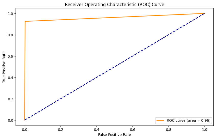
Accuracy: 0.91
Precision: 0.59
Recall: 0.96
F1 Score: 0.73
AUC: 0.93

Conclusiones#
a continuación se resumen todas las métricas obtenidas de los modelos de clasificación:
import pandas as pd
import matplotlib.pyplot as plt
import seaborn as sns

# Crear el dataframe con los datos
data = {
    'Modelo': ['LSTM', 'LSTM con SMOTE', 'KNN', 'KNN con SMOTE', 'Ridge', 'Ridge con SMOTE',
               'Naive Bayes', 'Naive Bayes con SMOTE', 'Random Forest', 'Random Forest con SMOTE',
               'Stacked Model', 'Stacked Model con SMOTE'],
    'Accuracy': [0.99, 0.91, 0.88, 0.82, 0.87, 0.78, 0.79, 0.79, 0.93, 0.86, 0.99, 0.91],
    'Precision': [0.98, 0.58, 0.55, 0.39, 0.42, 0.33, 0.33, 0.35, 0.87, 0.48, 0.98, 0.59],
    'Recall': [0.93, 0.95, 0.43, 0.71, 0.12, 0.65, 0.65, 0.71, 0.51, 0.80, 0.93, 0.96],
    'F1-score': [0.96, 0.72, 0.48, 0.50, 0.19, 0.44, 0.44, 0.47, 0.65, 0.60, 0.95, 0.73],
    'AUC': [0.97, 0.93, 0.69, 0.77, 0.55, 0.73, 0.73, 0.76, 0.75, 0.84, 0.96, 0.93]
}

df = pd.DataFrame(data)

# Crear el heatmap
plt.figure(figsize=(10, 8))
sns.set(font_scale=1)
sns.heatmap(df.set_index('Modelo'), cmap='RdYlGn', annot=True, fmt=".2f", linewidths=.5)
plt.title('Metricas de Modelos utilizados para la Clasificación')
plt.show()
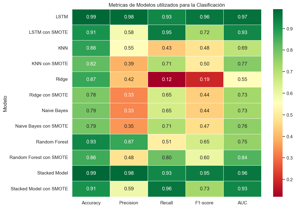
Modelado y Desempeño: La utilización del enfoque Doc2Vec para representar los mensajes en forma de vectores fue un paso determinante en la obtención de un modelo bastante efectivo para la tarea de clasificación de correos, permitiendo que los mensajes se convirtieran en entradas adecuadas para el modelo de deep learning. La elección de una red LSTM para la clasificación de mensajes demostró ser adecuada, dada la naturaleza secuencial del texto. Durante el entrenamiento, el modelo demostró una capacidad impresionante para adaptarse a los datos, logrando una precisión casi perfecta, además de superar por mucho a los modelos de machine learning clásicos empleados para esta tarea.
La técnica SMOTE demuestra no ser muy útil para mejorar las métricas del modelo LSTM para clasificar los correos, sin embargo, esta técnica sí favorece al performance de modelos de machine learning clásicos tales como KNN, Ridge y Random Forest. Adicionalmente, la técnica ha demostrado no ser tán efectiva en problemas de NLP tanto como lo es en problemas de regresión.
Modelo Stacked: El modelo Stacked usando la red neuronal con LSTM y KNN demuestra no tener un mal performance, sin embargo no supera a la técnica LSTM por sí sola, sin embargo, al evaluar la métrica de RECALL, se evidencia que el Stacked Model con SMOTE es el modelo que mejor RECALL posee de todos.