Mathematical functions for data science & artificial intelligence#
Algebraic functions#
Linear functions#
Tiene la forma de $\(f(x)=mx + b\)\( donde \)m\( y \)b\( \)\in R$.
\(m\) puede ser calculada por: $\(m=\frac{y_{2}-y_{1}}{x_{2}-x_{1}}\)$
y \(b\) es el punto de corte con el eje \(y\). Su dominio es \(Dom_{f} = (-\infty, \infty)\). Su imagen es \(Im_{f} = (-\infty, \infty)\)
coding a linear function#
import numpy as np
import matplotlib.pyplot as plt

N = 100

#slope
m = -1

#intercept
b = 3

#let's define the function
def f(x):
  return (m*x + b)

#domain
x = np.linspace(-10,10, num=N)

#range
y = f(x)

fig, ax = plt.subplots()
ax.plot(x,y)
ax.grid()
---------------------------------------------------------------------------
ModuleNotFoundError                       Traceback (most recent call last)
Cell In[1], line 2
      1 import numpy as np
----> 2 import matplotlib.pyplot as plt
      4 N = 100
      6 #slope

ModuleNotFoundError: No module named 'matplotlib'
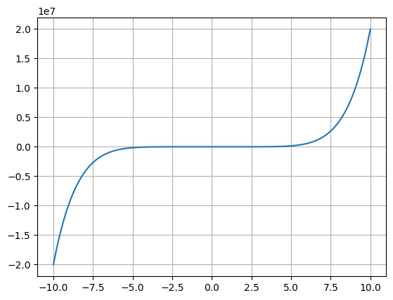
Polinomic functions#
Tiene la forma de $\(P(x)=a_{n}x^{n} + a_{n-1}x^{n-1}+...+a_{2}x^{2}+a_{1}x + a_{1}\)$
a una función que tiene esta forma se le llama polinomio de grado \(n\). A los elementos \(a\) los llamaremos coeficientes donde \(a \in R\).
Por ejemplo:
que es un polinomio de grado 7.
def f2(x):
    return(2*(x**7) - x**4 + 3*(x**2) + 4)

y2 = f2(x)

fig, ax2 = plt.subplots()
ax2.plot(x,y2)
ax2.grid()
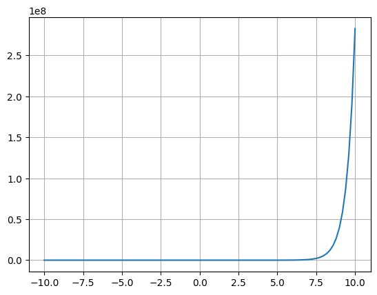
Power Function#
Hay unas funciones que son un caso particular de las funciones polinómicas que son las funciones potencia, las cuales tienen la forma:
Por ejemplo:
El dominio de \(f(x)=x^{2}\) es \(Dom_{f} = (-\infty, \infty)\). Su imagen es \(Im_{f} = [0, \infty)\)
Coding a power function#
def f3(x):
  return 7**x

y3 = f3(x)

fig, ax3 = plt.subplots()
ax3.plot(x,y3)
ax3.grid()
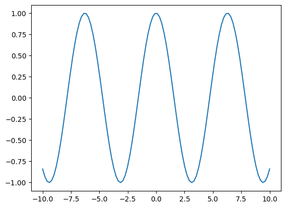
Trascendent functions#
these are functions that cannot be expressed as polynomials
Trigonometric functions#
def f(x):
  return np.cos(x)

y = f(x)

plt.plot(x,y)
[<matplotlib.lines.Line2D at 0x7f7f7b89f4c0>]
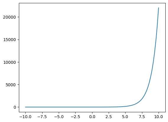
Exponential function#
Tienen la forma de $\(f(x)=a^x\)\( donde la base \)a$ es una constante positiva. Un gran ejemplo de una función exponencial es usando la base como el número de euler:
def f(x):
  return np.exp(x)    #euler

y=f(x)

plt.plot(x,y)
[<matplotlib.lines.Line2D at 0x7f7f7b82c4c0>]
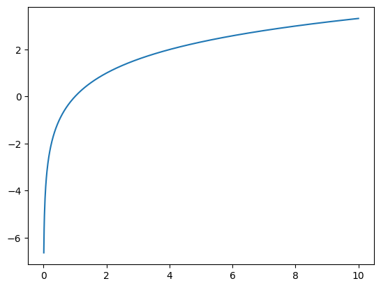
Logarithmic functions#
El logaritmo está definido por la relación:
donde:
\(b\) es la base.
\(n\) es el exponente al que está elevado la base.
\(x\) es el resultado de elevar la base \(b\) al exponente \(n\)
Ejemplo:
Teniendo b=2 y n=8, entonces:
Por lo que \(x=256\). Calculando el logaritmo base 2 de \(x\) es:
def f(x):
    return np.log2(x)

#domain
x = np.linspace(0, 10, 1000)

plt.plot(x, f(x))
plt.show()
/tmp/ipykernel_224/3839064836.py:2: RuntimeWarning: divide by zero encountered in log2
  return np.log2(x)
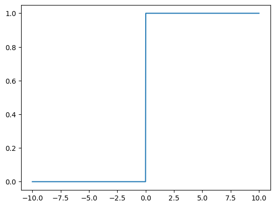
Heavyside function#
Son funciones que tienen diferentes valores definidos por un intervalo. Por ejemplo la función escalón de Heaviside:
x = np.linspace(-10, 10, 1000)

def f(x):

    Y = np.zeros(len(x))

    for index, x in enumerate(x):
        if x >= 0:
            Y[index] = 1
    return Y

plt.plot(x, f(x))
plt.show
<function matplotlib.pyplot.show(close=None, block=None)>
x = np.linspace(-3, 3, 7)

#if you want to understand the enumerate:

type(enumerate(x))

for index, x in enumerate(x):
    print("index is:", index)
    print("value is:", x)
index is: 0
value is: -3.0
index is: 1
value is: -2.0
index is: 2
value is: -1.0
index is: 3
value is: 0.0
index is: 4
value is: 1.0
index is: 5
value is: 2.0
index is: 6
value is: 3.0
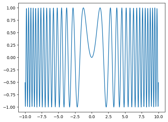
Composite functions#
import numpy as np
import matplotlib.pyplot as plt

N = 1000

x = np.linspace(-10,10, num=N)

def g(x):
  return x**2

def f(x):
  return np.sin(x)

y = g(x)

#this is basically plotting sin(x^2)
f_o_g = f(g(x))

plt.plot(x,f_o_g)
[<matplotlib.lines.Line2D at 0x7f7f7b7b30a0>]
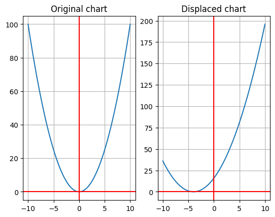
How to manipulate functions#
Functions displacement#
Siendo \(c\) una constante mayor que cero, entonces la gráfica:
\(y=f(x)+c\) se desplaza \(c\) unidades hacia arriba.
\(y=f(x)-c\) se desplaza \(c\) unidades hacia abajo.
\(y=f(x-c)\) se desplaza \(c\) unidades hacia la derecha.
\(y=f(x+c)\) se desplaza \(c\) unidades hacia la izquierda.
N = 1000

def f(x):
  return x**2;

c = 4

x = np.linspace(-10,10, num=N)

y = f(x + c)     #note that this will displace y 4 units to the right

fig, ax = plt.subplots(nrows=1, ncols=2)

ax[0].plot(x, f(x))     #original cuadratic function
ax[0].grid()
ax[0].axhline(y=0, color='r')
ax[0].axvline(x=0, color='r')
ax[0].set_title("Original chart")

ax[1].plot(x,y)         #function with transformation
ax[1].grid()
ax[1].axhline(y=0, color='r')
ax[1].axvline(x=0, color='r')
ax[1].set_title("Displaced chart")
Text(0.5, 1.0, 'Displaced chart')
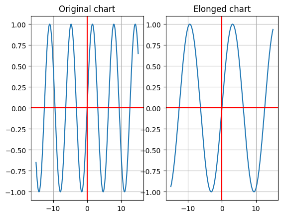
Functions elongations & compressions#
Siendo \(c\) una constante mayor que cero, entonces la gráfica:
\(y=c \cdot f(x)\) alarga la gráfica verticalmente en un factor de \(c\).
\(y= \frac{1}{c} \cdot f(x)\) comprime la gráfica verticalmente en un factor de \(c\).
\(y=f(c \cdot x)\) comprime la gráfica horizontelmente en un factor de \(c\).
\(y= f(\frac{1}{c} \cdot x )\) alarga la gráfica horizontelmente en un factor de \(c\).
N = 1000

def f(x):
  return np.sin(x);

c = 2

x = np.linspace(-15,15, num=N)

y = f((1/c)*x)     #note that this will elonge the chart in a proportion of 2


fig, ax = plt.subplots(nrows=1, ncols=2)

ax[0].plot(x, f(x))     #original sinusoidal function
ax[0].grid()
ax[0].axhline(y=0, color='r')
ax[0].axvline(x=0, color='r')
ax[0].set_title("Original chart")

ax[1].plot(x,y)         #function with transformation (elonged horizontally)
ax[1].grid()
ax[1].axhline(y=0, color='r')
ax[1].axvline(x=0, color='r')
ax[1].set_title("Elonged chart")
Text(0.5, 1.0, 'Elonged chart')
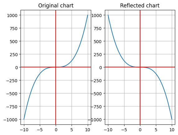
Function reflection#
\(y=-f(x)\) refleja la gráfica respecto al eje x.
\(y=f(-x)\) refleja la gráfica respecto al eje y.
N = 1000

def f(x):
  return x**3;

x = np.linspace(-10,10, num=N)

y = f(-x)      #this will reflect the function about the y axis

fig, ax = plt.subplots(nrows=1, ncols=2)

ax[0].plot(x, f(x))     #original cubic function
ax[0].grid()
ax[0].axhline(y=0, color='r')
ax[0].axvline(x=0, color='r')
ax[0].set_title("Original chart")

ax[1].plot(x,y)         #function with transformation (reflected about the y axis)
ax[1].grid()
ax[1].axhline(y=0, color='r')
ax[1].axvline(x=0, color='r')
ax[1].set_title("Reflected chart")
Text(0.5, 1.0, 'Reflected chart')
Activation Functions#
import numpy as np
import matplotlib.pyplot as plt

N = 1000
x = np.linspace(-5,5, num=N)
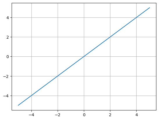
Linear function#
def f(x):
  return x

plt.plot(x, f(x))
plt.grid()
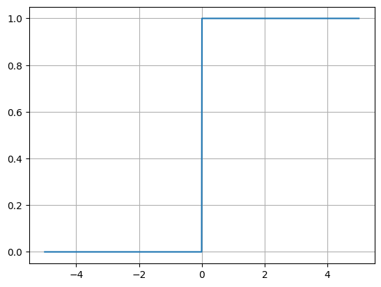
heavyside function#
def H(x):
  Y = np.zeros(len(x))
  for idx,x in enumerate(x):
    if x>=0:
      Y[idx]=1
  return Y


N=1000


y = H(x)

plt.plot(x,y)
plt.grid()
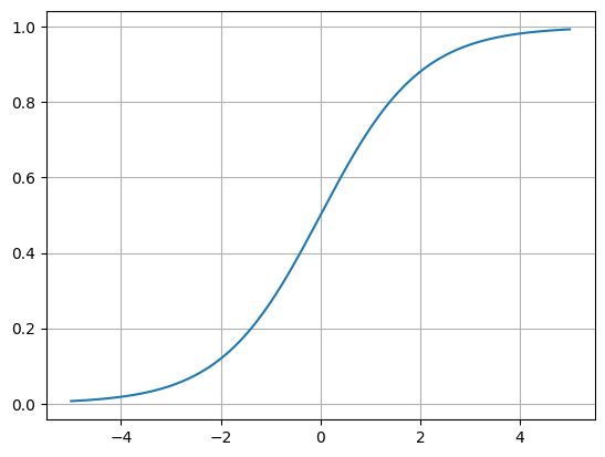
sigmoid function#
def f(x):
  return 1/(1 + np.exp(-x))


N=1000

y = f(x)

plt.plot(x,y)
plt.grid()
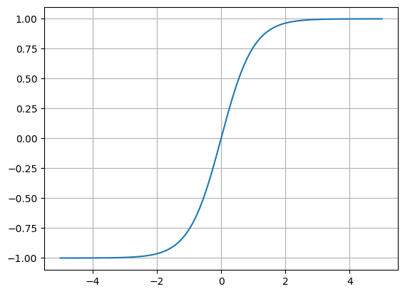
hyperbolic tangent function#
def f(x):
  return np.tanh(x)


N=1000

y = f(x)

plt.plot(x,y)
plt.grid()
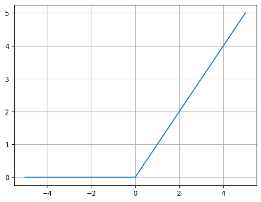
ReLu function#
def f(x):
  return np.maximum(x,0)


N=1000

y = f(x)

plt.plot(x,y)
plt.grid()
 Created in Deepnote