Manejo de Datos Faltantes: Detección

Preparacion de entorno

pip install -r requirements.txt

^C
Requirement already satisfied: pip in c:\users\admin\miniconda3\lib\site-packages (from -r requirements.txt (line 1)) (23.1.2)
Collecting pyjanitor (from -r requirements.txt (line 2))
  Using cached pyjanitor-0.25.0-py3-none-any.whl (171 kB)
Collecting missingno (from -r requirements.txt (line 3))
  Using cached missingno-0.5.2-py3-none-any.whl (8.7 kB)
Requirement already satisfied: numpy in c:\users\admin\miniconda3\lib\site-packages (from -r requirements.txt (line 4)) (1.25.2)
Collecting matplotlib==3.5.1 (from -r requirements.txt (line 5))
  Using cached matplotlib-3.5.1.tar.gz (35.3 MB)
  Preparing metadata (setup.py): started
  Preparing metadata (setup.py): finished with status 'done'
Requirement already satisfied: pandas in c:\users\admin\miniconda3\lib\site-packages (from -r requirements.txt (line 6)) (2.1.0)
Collecting pyreadr (from -r requirements.txt (line 7))
  Using cached pyreadr-0.4.9-cp311-cp311-win_amd64.whl (1.3 MB)
Requirement already satisfied: seaborn in c:\users\admin\miniconda3\lib\site-packages (from -r requirements.txt (line 8)) (0.12.2)
Collecting session-info (from -r requirements.txt (line 9))
  Using cached session_info-1.0.0.tar.gz (24 kB)
  Preparing metadata (setup.py): started
  Preparing metadata (setup.py): finished with status 'done'
Collecting upsetplot==0.6.1 (from -r requirements.txt (line 10))
  Using cached UpSetPlot-0.6.1.tar.gz (18 kB)
  Preparing metadata (setup.py): started
  Preparing metadata (setup.py): finished with status 'done'
Requirement already satisfied: cycler>=0.10 in c:\users\admin\miniconda3\lib\site-packages (from matplotlib==3.5.1->-r requirements.txt (line 5)) (0.11.0)
Requirement already satisfied: fonttools>=4.22.0 in c:\users\admin\miniconda3\lib\site-packages (from matplotlib==3.5.1->-r requirements.txt (line 5)) (4.42.1)
Requirement already satisfied: kiwisolver>=1.0.1 in c:\users\admin\miniconda3\lib\site-packages (from matplotlib==3.5.1->-r requirements.txt (line 5)) (1.4.5)
Requirement already satisfied: packaging>=20.0 in c:\users\admin\miniconda3\lib\site-packages (from matplotlib==3.5.1->-r requirements.txt (line 5)) (23.0)
Requirement already satisfied: pillow>=6.2.0 in c:\users\admin\miniconda3\lib\site-packages (from matplotlib==3.5.1->-r requirements.txt (line 5)) (10.0.0)
Requirement already satisfied: pyparsing>=2.2.1 in c:\users\admin\miniconda3\lib\site-packages (from matplotlib==3.5.1->-r requirements.txt (line 5)) (3.0.9)
Requirement already satisfied: python-dateutil>=2.7 in c:\users\admin\miniconda3\lib\site-packages (from matplotlib==3.5.1->-r requirements.txt (line 5)) (2.8.2)
Collecting natsort (from pyjanitor->-r requirements.txt (line 2))
  Downloading natsort-8.4.0-py3-none-any.whl (38 kB)
Requirement already satisfied: pandas-flavor in c:\users\admin\miniconda3\lib\site-packages (from pyjanitor->-r requirements.txt (line 2)) (0.6.0)
Collecting multipledispatch (from pyjanitor->-r requirements.txt (line 2))
  Downloading multipledispatch-1.0.0-py3-none-any.whl (12 kB)
Requirement already satisfied: scipy in c:\users\admin\miniconda3\lib\site-packages (from pyjanitor->-r requirements.txt (line 2)) (1.11.2)
Requirement already satisfied: pytz>=2020.1 in c:\users\admin\miniconda3\lib\site-packages (from pandas->-r requirements.txt (line 6)) (2023.3.post1)
Requirement already satisfied: tzdata>=2022.1 in c:\users\admin\miniconda3\lib\site-packages (from pandas->-r requirements.txt (line 6)) (2023.3)
Collecting stdlib_list (from session-info->-r requirements.txt (line 9))
  Downloading stdlib_list-0.9.0-py3-none-any.whl (75 kB)
                                              0.0/75.6 kB ? eta -:--:--
     ---------------------------------------- 75.6/75.6 kB 2.1 MB/s eta 0:00:00
Requirement already satisfied: six>=1.5 in c:\users\admin\miniconda3\lib\site-packages (from python-dateutil>=2.7->matplotlib==3.5.1->-r requirements.txt (line 5)) (1.16.0)
Requirement already satisfied: xarray in c:\users\admin\miniconda3\lib\site-packages (from pandas-flavor->pyjanitor->-r requirements.txt (line 2)) (2023.8.0)
Building wheels for collected packages: matplotlib, upsetplot, session-info
  Building wheel for matplotlib (setup.py): started

Note: you may need to restart the kernel to use updated packages.

Importar librerías

import janitor
import matplotlib.pyplot as plt
import missingno
import numpy as np
import pandas as pd
import pyreadr
import seaborn as sns
import session_info
import upsetplot

Importar funciones personalizadas

%run pandas-missing-extension.ipynb

Configurar el aspecto general de las gráficas del proyecto

%matplotlib inline

sns.set(
    rc={
        "figure.figsize": (10, 10)
    }
)

sns.set_style("whitegrid")

Cargar los conjuntos de datos

Pima Indians Diabetes

# Saving the link into a variable
pima_indians_diabetes_url = "https://nrvis.com/data/mldata/pima-indians-diabetes.csv"

# Downloading the csv file
!wget -O ./data/pima-indians-diabetes.csv { pima_indians_diabetes_url } -q

diabetes_df = pd.read_csv(
    "./data/pima-indians-diabetes.csv",
    sep=",",
    names=[
        "pregnancies",
        "glucose",
        "blood_pressure",
        "skin_thickness",
        "insulin",
        "bmi",
        "diabetes_pedigree_function",
        "age",
        "outcome",
    ]
)

diabetes_df.head()

	pregnancies	glucose	blood_pressure	skin_thickness	insulin	bmi	diabetes_pedigree_function	age	outcome
0	6	148	72	35	0	33.6	0.627	50	1
1	1	85	66	29	0	26.6	0.351	31	0
2	8	183	64	0	0	23.3	0.672	32	1
3	1	89	66	23	94	28.1	0.167	21	0
4	0	137	40	35	168	43.1	2.288	33	1

naniar (oceanbuoys, pedestrian, riskfactors)

Crear unidades de información de los conjuntos de datos

base_url = "https://github.com/njtierney/naniar/raw/master/data/"
dataset_names = ("oceanbuoys", "pedestrian", "riskfactors")
extension = ".rda"

Descargar y cargar los conjuntos de datos

datasets_dfs = {}

for dataset_name in dataset_names:

    dataset_file = f"{ dataset_name }{ extension }"
    dataset_output_file = f"./data/{ dataset_file }"
    dataset_url = f"{ base_url }{ dataset_file }"

    !wget -q -O { dataset_output_file } { dataset_url }

    datasets_dfs[f"{ dataset_name }_df"] = pyreadr.read_r(dataset_output_file).get(dataset_name)

datasets_dfs.keys()

dict_keys(['oceanbuoys_df', 'pedestrian_df', 'riskfactors_df'])

Incluir conjuntos de datos en nuestro ambiente local

locals().update(**datasets_dfs)
del datasets_dfs

Verificar carga

oceanbuoys_df.shape, pedestrian_df.shape, riskfactors_df.shape, diabetes_df.shape

((736, 8), (37700, 9), (245, 34), (768, 9))

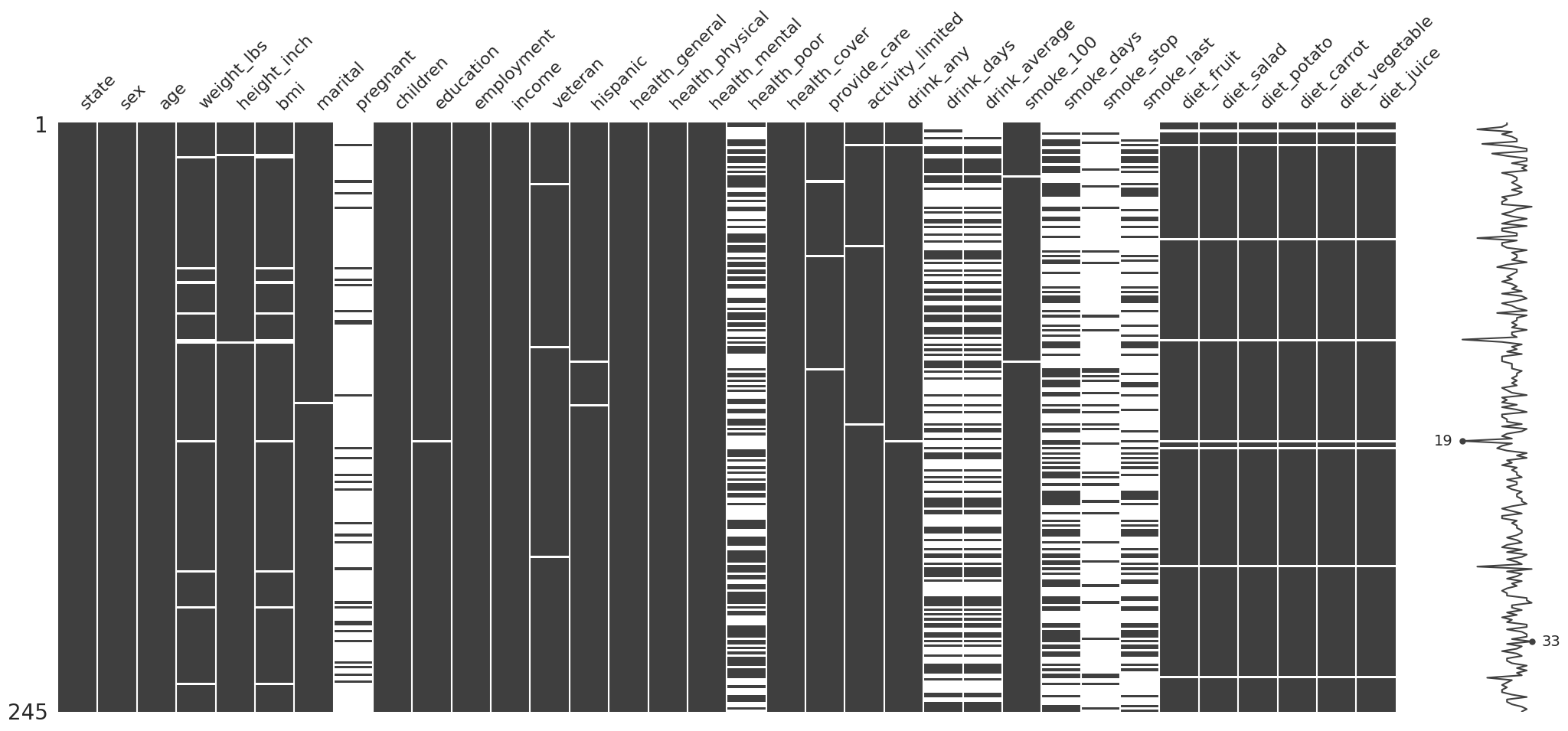
Note que la variable state tiene 245 valores no nulos, mientras que la variable pregnant tiene 30

la variable pregnant parece tener muchos valores no nulos, vamos a investigar?

riskfactors_df.info()

<class 'pandas.core.frame.DataFrame'>
RangeIndex: 245 entries, 0 to 244
Data columns (total 34 columns):
 #   Column            Non-Null Count  Dtype   
---  ------            --------------  -----   
 0   state             245 non-null    category
 1   sex               245 non-null    category
 2   age               245 non-null    int32   
 3   weight_lbs        235 non-null    object  
 4   height_inch       243 non-null    object  
 5   bmi               234 non-null    float64 
 6   marital           244 non-null    category
 7   pregnant          30 non-null     category
 8   children          245 non-null    int32   
 9   education         244 non-null    category
 10  employment        245 non-null    category
 11  income            245 non-null    category
 12  veteran           242 non-null    category
 13  hispanic          243 non-null    category
 14  health_general    245 non-null    category
 15  health_physical   245 non-null    int32   
 16  health_mental     245 non-null    int32   
 17  health_poor       132 non-null    object  
 18  health_cover      245 non-null    category
 19  provide_care      242 non-null    category
 20  activity_limited  242 non-null    category
 21  drink_any         243 non-null    category
 22  drink_days        111 non-null    object  
 23  drink_average     110 non-null    object  
 24  smoke_100         243 non-null    category
 25  smoke_days        117 non-null    category
 26  smoke_stop        33 non-null     category
 27  smoke_last        84 non-null     category
 28  diet_fruit        237 non-null    object  
 29  diet_salad        237 non-null    object  
 30  diet_potato       237 non-null    object  
 31  diet_carrot       237 non-null    object  
 32  diet_vegetable    237 non-null    object  
 33  diet_juice        237 non-null    object  
dtypes: category(18), float64(1), int32(4), object(11)
memory usage: 36.7+ KB

Tabulación de valores faltantes

Número total de valores completos (sin observaciones faltantes)

riskfactors_df.missing.number_complete()

7144

Número total de valores faltantes

riskfactors_df.missing.number_missing()

1186

Resúmenes tabulares de valores faltantes

Variables / Columnas

Resumen por variable

riskfactors_df.missing.missing_variable_summary()

	variable	n_missing	n_cases	pct_missing
0	state	0	245	0.000000
1	sex	0	245	0.000000
2	age	0	245	0.000000
3	weight_lbs	10	245	4.081633
4	height_inch	2	245	0.816327
5	bmi	11	245	4.489796
6	marital	1	245	0.408163
7	pregnant	215	245	87.755102
8	children	0	245	0.000000
9	education	1	245	0.408163
10	employment	0	245	0.000000
11	income	0	245	0.000000
12	veteran	3	245	1.224490
13	hispanic	2	245	0.816327
14	health_general	0	245	0.000000
15	health_physical	0	245	0.000000
16	health_mental	0	245	0.000000
17	health_poor	113	245	46.122449
18	health_cover	0	245	0.000000
19	provide_care	3	245	1.224490
20	activity_limited	3	245	1.224490
21	drink_any	2	245	0.816327
22	drink_days	134	245	54.693878
23	drink_average	135	245	55.102041
24	smoke_100	2	245	0.816327
25	smoke_days	128	245	52.244898
26	smoke_stop	212	245	86.530612
27	smoke_last	161	245	65.714286
28	diet_fruit	8	245	3.265306
29	diet_salad	8	245	3.265306
30	diet_potato	8	245	3.265306
31	diet_carrot	8	245	3.265306
32	diet_vegetable	8	245	3.265306
33	diet_juice	8	245	3.265306

Tabulación del resumen por variable

riskfactors_df.missing.missing_variable_table()

	n_missing_in_variable	n_variables	pct_variables
0	0	10	29.411765
1	8	6	17.647059
2	2	4	11.764706
3	3	3	8.823529
4	1	2	5.882353
5	10	1	2.941176
6	11	1	2.941176
7	113	1	2.941176
8	128	1	2.941176
9	134	1	2.941176
10	135	1	2.941176
11	161	1	2.941176
12	212	1	2.941176
13	215	1	2.941176

Casos / Observaciones / Filas

Resúmenes por caso (muestra valores nulos por row)

riskfactors_df.missing.missing_case_summary()

	case	n_missing	pct_missing
0	0	6	16.666667
1	1	6	16.666667
2	2	7	19.444444
3	3	12	33.333333
4	4	5	13.888889
...	...	...	...
240	240	6	16.666667
241	241	5	13.888889
242	242	3	8.333333
243	243	2	5.555556
244	244	3	8.333333

245 rows × 3 columns

Tabulación del resumen por caso

riskfactors_df.missing.missing_case_table()

	n_missing_in_case	n_cases	pct_case
0	4	49	20.000000
1	5	45	18.367347
2	7	39	15.918367
3	6	36	14.693878
4	2	31	12.653061
5	3	30	12.244898
6	1	4	1.632653
7	8	3	1.224490
8	12	3	1.224490
9	15	2	0.816327
10	9	1	0.408163
11	10	1	0.408163
12	11	1	0.408163

Intervalos de valores faltantes

(
    riskfactors_df
    .missing
    .missing_variable_span(
        variable="weight_lbs",            # variable a analizar
        span_every=50                     # intervalos a romper la variable
    )
)

	span_counter	n_missing	n_complete	pct_missing	pct_complete
0	0	1	49	2.000000	98.000000
1	1	5	45	10.000000	90.000000
2	2	1	49	2.000000	98.000000
3	3	1	49	2.000000	98.000000
4	4	2	43	4.444444	95.555556

Run length de valores faltantes

Detecta automáticamente el conteo seguido de variables nulas

(
    riskfactors_df
    .missing
    .missing_variable_run(
        variable="weight_lbs"
    )
)

	run_length	is_na
0	14	complete
1	1	missing
2	45	complete
3	1	missing
4	5	complete
5	1	missing
6	12	complete
7	1	missing
8	10	complete
9	2	missing
10	40	complete
11	1	missing
12	53	complete
13	1	missing
14	14	complete
15	1	missing
16	31	complete
17	1	missing
18	11	complete

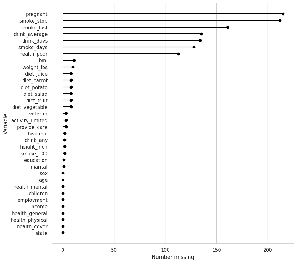
Visualización inicial de valores faltantes

Variable

riskfactors_df.missing.missing_variable_plot()

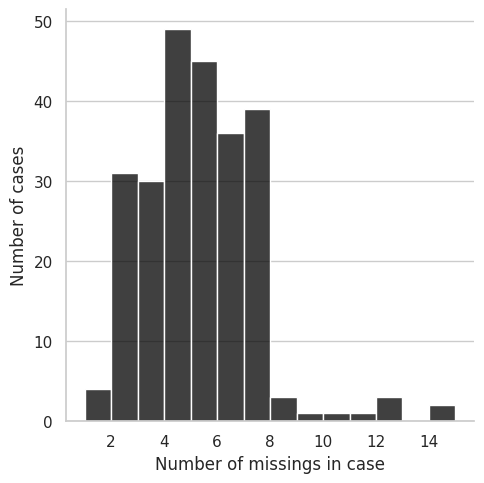
Casos / Observaciones / Filas

riskfactors_df.missing.missing_case_plot()

(
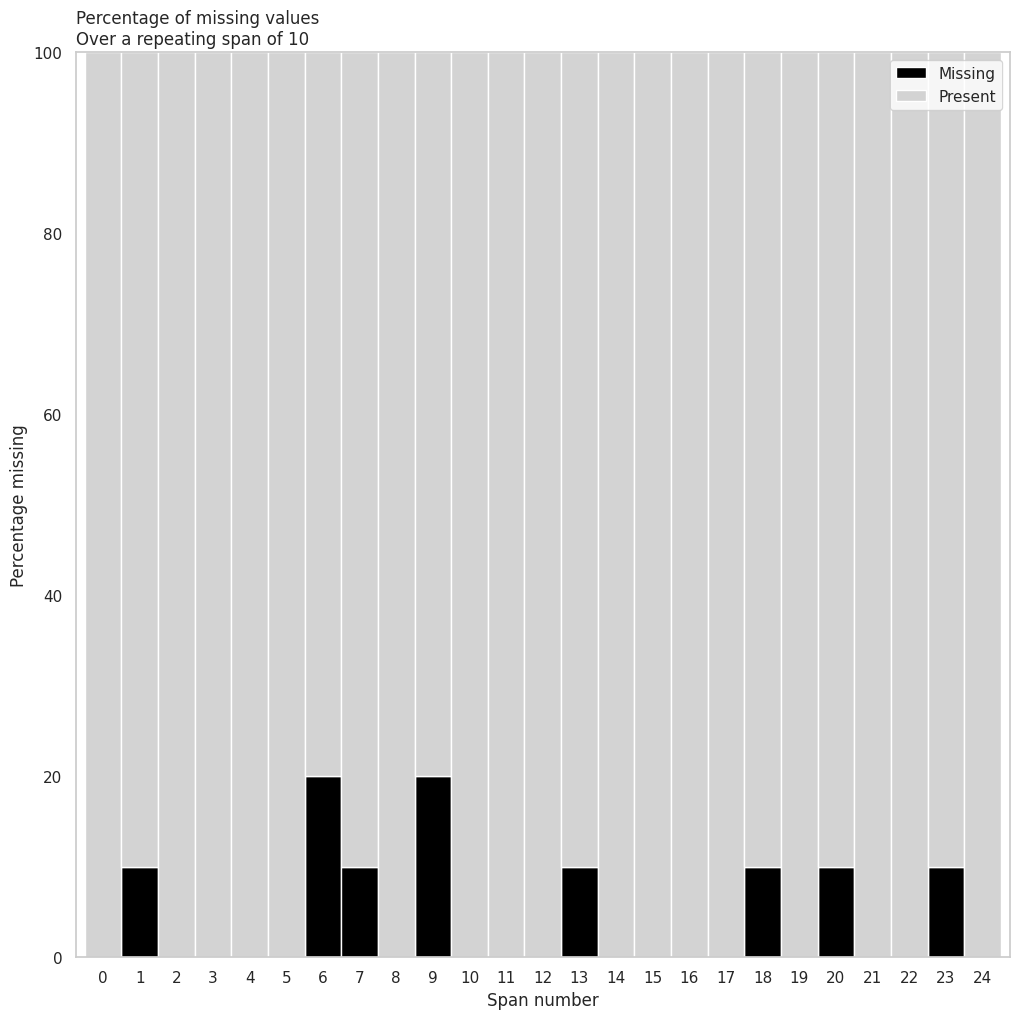
    riskfactors_df
    .missing
    .missing_variable_span_plot(
        variable="weight_lbs",
        span_every=10,
        rot = 0     # label rotation
    )
)

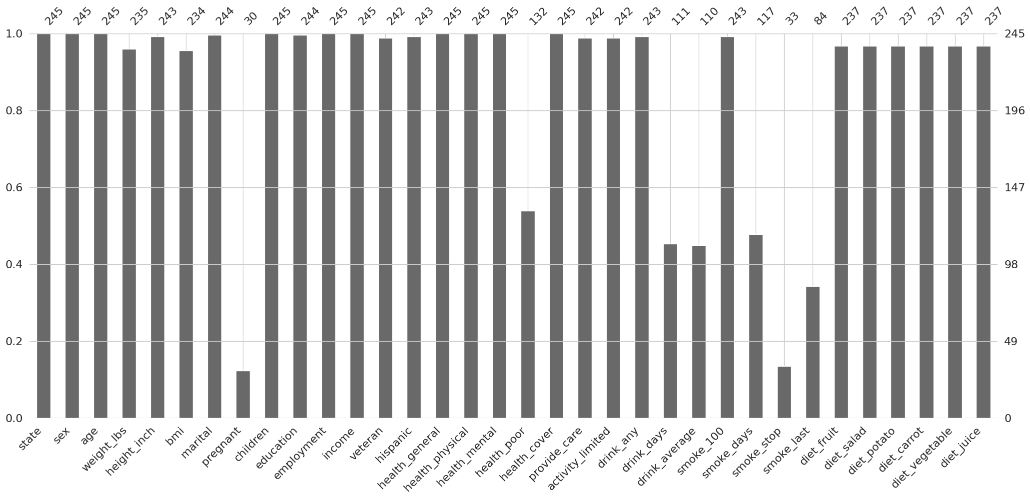
Que tan completas están nuestras variables?

missingno.bar(df = riskfactors_df);

missingno.matrix(df=riskfactors_df);

/root/venv/lib/python3.9/site-packages/missingno/missingno.py:73: MatplotlibDeprecationWarning: The 'b' parameter of grid() has been renamed 'visible' since Matplotlib 3.5; support for the old name will be dropped two minor releases later.
  ax0.grid(b=False)
/root/venv/lib/python3.9/site-packages/missingno/missingno.py:142: MatplotlibDeprecationWarning: The 'b' parameter of grid() has been renamed 'visible' since Matplotlib 3.5; support for the old name will be dropped two minor releases later.
  ax1.grid(b=False)

(
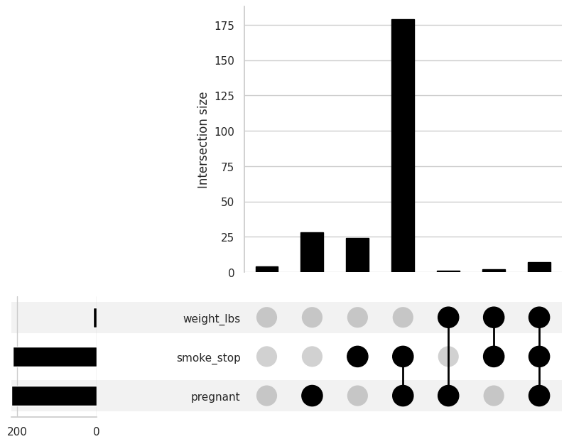
    riskfactors_df
    .missing
    .missing_upsetplot(
        variables=["pregnant","weight_lbs","smoke_stop"],  # Put the target variable name
        # alternatively, put none to see all variables
        
        element_size = 60    # This one specifies the size of the figure that you want to create
    )
);

Codificación de valores faltantes

🚧 Advertencia

Al igual que cada persona es una nueva puerta a un mundo diferente, los valores faltantes existen en diferentes formas y colores. Al trabajar con valores faltantes será crítico entender sus distintas representaciones. A pesar de que el conjunto de datos de trabajo pareciera que no contiene valores faltantes, deberás ser capaz de ir más allá de lo observado a simple vista para remover el manto tras el cual se esconde lo desconocido.

Valores comúnmente asociados a valores faltantes

Cadenas de texto

common_na_strings = (
    "missing",
    "NA",
    "N A",
    "N/A",
    "#N/A",
    "NA ",
    " NA",
    "N /A",
    "N / A",
    " N / A",
    "N / A ",
    "na",
    "n a",
    "n/a",
    "na ",
    " na",
    "n /a",
    "n / a",
    " a / a",
    "n / a ",
    "NULL",
    "null",
    "",
    "?",
    "*",
    ".",
)

Números

common_na_numbers = (-9, -99, -999, -9999, 9999, 66, 77, 88, -1)

¿Cómo encontrar los valores comúnmente asociados a valores faltantes?

missing_data_example_df = pd.DataFrame.from_dict(
    dict(
        x = [1, 3, "NA", -99, -98, -99],
        y = ["A", "N/A", "NA", "E", "F", "G"],
        z = [-100, -99, -98, -101, -1, -1]
    )
)

missing_data_example_df

	x	y	z
0	1	A	-100
1	3	N/A	-99
2	NA	NA	-98
3	-99	E	-101
4	-98	F	-1
5	-99	G	-1

Ya sabemos que hay valores faltantes

Será que Pandas los detecta?

missing_data_example_df.isna()

	x	y	z
0	False	False	False
1	False	False	False
2	False	False	False
3	False	False	False
4	False	False	False
5	False	False	False

Sustituyendo valores comúnmente asociados a valores faltantes

Sustitución desde la lectura de datos

pd.read_csv(
    "./data/missing_data_enconding_example.csv",
    na_filter=True,
    na_values=[-99, -1]
)

	x	y	z
0	1.0	A	-100.0
1	3.0	NaN	NaN
2	NaN	NaN	-98.0
3	NaN	E	-101.0
4	-98.0	F	NaN
5	NaN	G	NaN

Sustitución global

(
    missing_data_example_df
    .replace(
        to_replace=[-99, "NA"],
        value=np.nan
    )
)

	x	y	z
0	1.0	A	-100.0
1	3.0	N/A	NaN
2	NaN	NaN	-98.0
3	NaN	E	-101.0
4	-98.0	F	-1.0
5	NaN	G	-1.0

Sustitución dirigida

Sustituir solamente en una columna

(
    missing_data_example_df
    .replace(
        to_replace={
            "x":{-99:np.nan}
        }
    )
)

	x	y	z
0	1	A	-100
1	3	N/A	-99
2	NA	NA	-98
3	NaN	E	-101
4	-98	F	-1
5	NaN	G	-1

Conversión de valores faltantes implícitos a explícitos

🚧 Advertencia

"Implícito se refiere a todo aquello que se entiende que está incluido pero sin ser expresado de forma directa o explícitamente."

Un valor faltante implícito indica que el valor faltante debería estar incluido en el conjunto de datos del análisis, sin que éste lo diga o lo especifique. Por lo general, son valores que podemos encontrar al pivotar nuestros datos o contabilizar el número de apariciones de combinaciones de las variables de estudio.

implicit_to_explicit_df = pd.DataFrame.from_dict(
    data={
        "name": ["lynn", "lynn", "lynn", "zelda"],
        "time": ["morning", "afternoon", "night", "morning"],
        "value": [350, 310, np.nan, 320]
    }
)

implicit_to_explicit_df

	name	time	value
0	lynn	morning	350.0
1	lynn	afternoon	310.0
2	lynn	night	NaN
3	zelda	morning	320.0

Note que implicitamente hay valores faltantes, por que zelda no tiene valores para afternoon & night?

Estrategias para la identificación de valores faltantes implícitos

Pivotar la tabla de datos

(
    implicit_to_explicit_df
    .pivot_wider(
        index="name",
        names_from="time",
        values_from="value"
    )
)

	name	afternoon	morning	night
0	lynn	310.0	350.0	NaN
1	zelda	NaN	320.0	NaN

Cuantificar ocurrencias de n-tuplas

(
    implicit_to_explicit_df
    .value_counts(
        subset=["name"]
    )
    .reset_index(name="n")
    .query("n<3")
)

	name	n
1	zelda	1

Exponer filas faltantes implícitas a explícitas

📘 Información

janitor.complete() está modelada a partir de la función complete() del paquete tidyr y es un wrapper alrededor de janitor.expand_grid(), pd.merge() y pd.fillna(). En cierto modo, es lo contrario de pd.dropna(), ya que expone implícitamente las filas que faltan.

Son posibles combinaciones de nombres de columnas o una lista/tupla de nombres de columnas, o incluso un diccionario de nombres de columna y nuevos valores.

Las columnas MultiIndex no son complatibles.

Exponer n-tuplas de valores faltantes

Ejemplo, encontrar los pares faltantes de name y time.

(
    implicit_to_explicit_df

    #janitor
    .complete(
        "name",
        "time"
    )
)

	name	time	value
0	lynn	morning	350.0
1	lynn	afternoon	310.0
2	lynn	night	NaN
3	zelda	morning	320.0
4	zelda	afternoon	NaN
5	zelda	night	NaN

Limitar la exposición de n-tuplas de valores faltantes

(
    implicit_to_explicit_df

    #janitor
    .complete(
        {"name":["lynn", "zelda"]},
        {"time":["morning", "afternoon"]},
        sort=True
    )
)

	name	time	value
0	lynn	afternoon	310.0
1	lynn	morning	350.0
2	zelda	afternoon	NaN
3	zelda	morning	320.0
4	lynn	night	NaN

Rellenar los valores faltantes

(
    implicit_to_explicit_df

    #janitor
    .complete(
        "name",
        "time",
        fill_value = np.nan    #aqui se puede poner cualquier valor para los nulos
    )
)

	name	time	value
0	lynn	morning	350.0
1	lynn	afternoon	310.0
2	lynn	night	NaN
3	zelda	morning	320.0
4	zelda	afternoon	NaN
5	zelda	night	NaN

Limitar el rellenado de valores faltantes implícitos

(
    implicit_to_explicit_df

    #janitor
    .complete(
        "name",
        "time",
        fill_value = 0,
        explicit=False
    )
)

	name	time	value
0	lynn	morning	350.0
1	lynn	afternoon	310.0
2	lynn	night	NaN
3	zelda	morning	320.0
4	zelda	afternoon	0.0
5	zelda	night	0.0

Tipos de valores faltantes

Usando el DF de diabetes, determine si hay valores faltantes

diabetes_df.missing.missing_variable_plot()

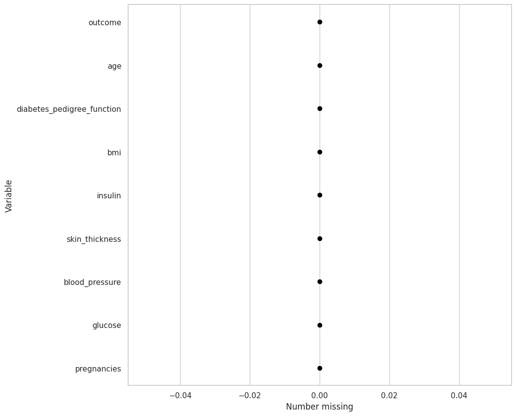
This chart is basically saying that there are no missing values, which is false. The problem is that the missing values are in a different format

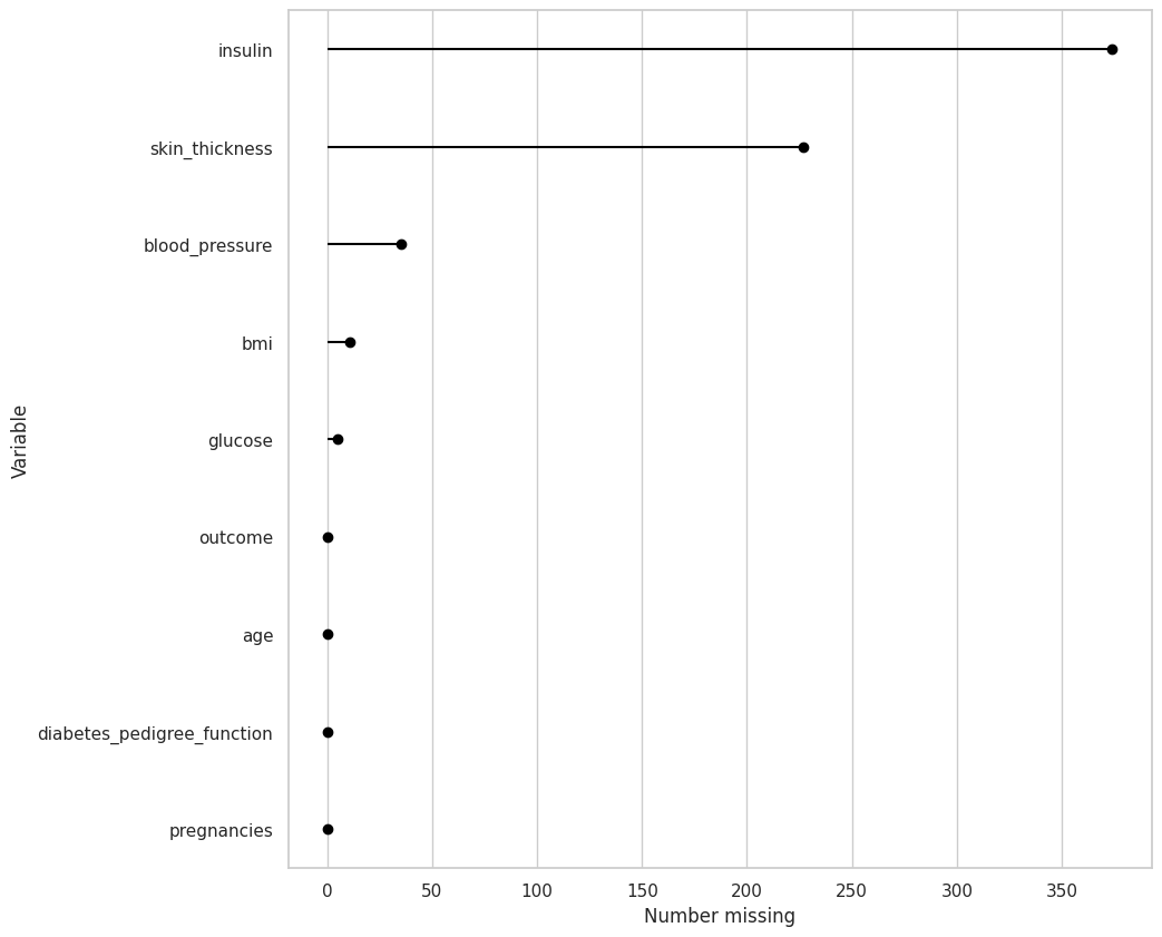
The missing values are shown as a zero, let’s change them into numpy nan

diabetes_df[diabetes_df.columns[1:6]] = diabetes_df[diabetes_df.columns[1:6]].replace(0, np.nan)
diabetes_df.missing.missing_variable_plot()

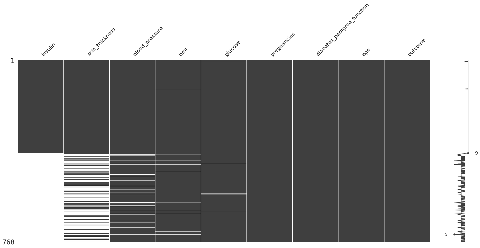
Missing Completely At Random (MCAR)

(
    diabetes_df
    .missing.sort_variables_by_missingness()
    .pipe(missingno.matrix)
)

/root/venv/lib/python3.9/site-packages/missingno/missingno.py:73: MatplotlibDeprecationWarning: The 'b' parameter of grid() has been renamed 'visible' since Matplotlib 3.5; support for the old name will be dropped two minor releases later.
  ax0.grid(b=False)
/root/venv/lib/python3.9/site-packages/missingno/missingno.py:142: MatplotlibDeprecationWarning: The 'b' parameter of grid() has been renamed 'visible' since Matplotlib 3.5; support for the old name will be dropped two minor releases later.
  ax1.grid(b=False)

<AxesSubplot:>

Se ordenan las columnas tal que las que tienen mas valores faltantes aparecen primero.

Missing At Random (MAR)

(
    diabetes_df
    .missing.sort_variables_by_missingness()
    .sort_values(by="blood_pressure")
    .pipe(missingno.matrix)
)

/root/venv/lib/python3.9/site-packages/missingno/missingno.py:73: MatplotlibDeprecationWarning: The 'b' parameter of grid() has been renamed 'visible' since Matplotlib 3.5; support for the old name will be dropped two minor releases later.
  ax0.grid(b=False)
/root/venv/lib/python3.9/site-packages/missingno/missingno.py:142: MatplotlibDeprecationWarning: The 'b' parameter of grid() has been renamed 'visible' since Matplotlib 3.5; support for the old name will be dropped two minor releases later.
  ax1.grid(b=False)

<AxesSubplot:>

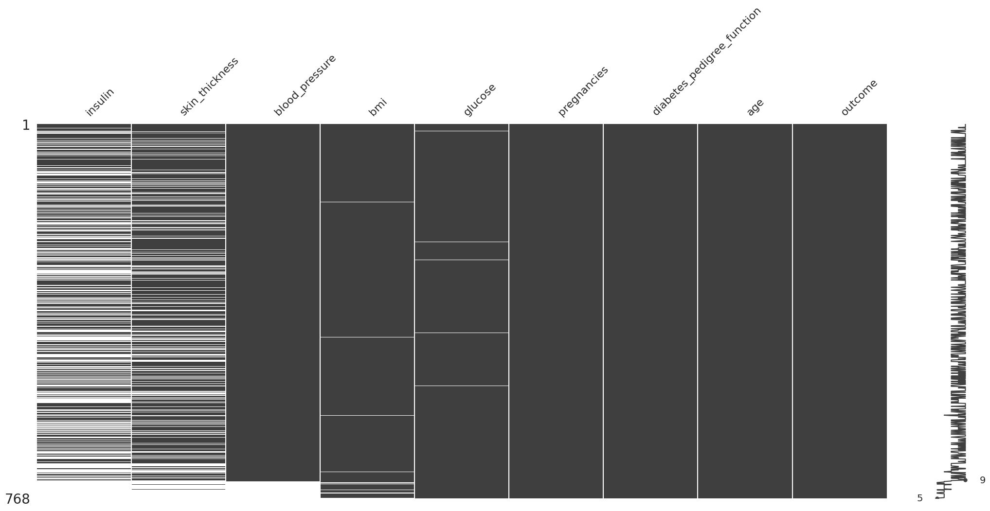
Aqui se puede empezar a inferir que puede haber una relacion entre la presion sanguinea y los datos faltantes

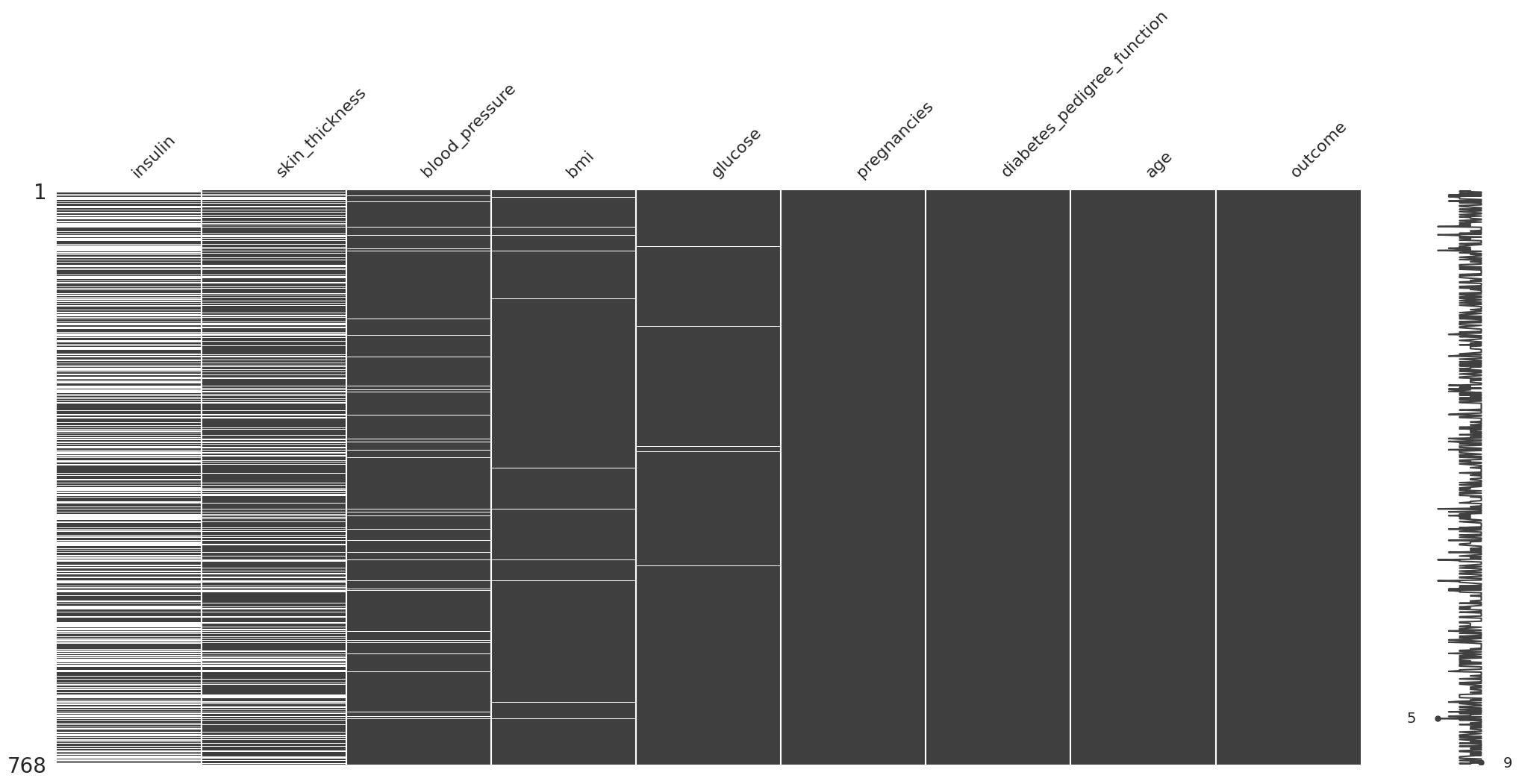
Missing Not At Random (MNAR)

(
    diabetes_df
    .missing.sort_variables_by_missingness()
    .sort_values(by="insulin")
    .pipe(missingno.matrix)
)

/root/venv/lib/python3.9/site-packages/missingno/missingno.py:73: MatplotlibDeprecationWarning: The 'b' parameter of grid() has been renamed 'visible' since Matplotlib 3.5; support for the old name will be dropped two minor releases later.
  ax0.grid(b=False)
/root/venv/lib/python3.9/site-packages/missingno/missingno.py:142: MatplotlibDeprecationWarning: The 'b' parameter of grid() has been renamed 'visible' since Matplotlib 3.5; support for the old name will be dropped two minor releases later.
  ax1.grid(b=False)

<AxesSubplot:>

Aqui podemos observar que este error es sistematico. Siempre que se colectan los datos de insulina, tambien se colectan el resto de datos. A su vez, cuando no se colectan los datos de insulina, tienden a haber datos faltantes en las otras variables

Concepto y aplicación de la matriz de sombras (i.e., shadow matrix)

Construcción de la matriz de sombras

(
    riskfactors_df
    .isna()
    .replace({
        False:"Not missing",
        True:"Missing"
    })
    .add_suffix("_NA")
    .pipe(
        lambda shadow_matrix: pd.concat(
            [riskfactors_df, shadow_matrix],
            axis="columns"
        )
    )
)

	state	sex	age	weight_lbs	height_inch	bmi	marital	pregnant	children	education	...	smoke_100_NA	smoke_days_NA	smoke_stop_NA	smoke_last_NA	diet_fruit_NA	diet_salad_NA	diet_potato_NA	diet_carrot_NA	diet_vegetable_NA	diet_juice_NA
0	26	Female	49	190	64	32.68	Married	NaN	0	6	...	Not missing	Missing	Missing	Missing	Not missing	Not missing	Not missing	Not missing	Not missing	Not missing
1	40	Female	48	170	68	25.90	Divorced	NaN	0	5	...	Not missing	Missing	Missing	Missing	Not missing	Not missing	Not missing	Not missing	Not missing	Not missing
2	72	Female	55	163	64	28.04	Married	NaN	0	4	...	Not missing	Missing	Missing	Missing	Not missing	Not missing	Not missing	Not missing	Not missing	Not missing
3	42	Male	42	230	74	29.59	Married	NaN	1	6	...	Not missing	Missing	Missing	Missing	Missing	Missing	Missing	Missing	Missing	Missing
4	32	Female	66	135	62	24.74	Widowed	NaN	0	5	...	Not missing	Not missing	Not missing	Missing	Not missing	Not missing	Not missing	Not missing	Not missing	Not missing
...	...	...	...	...	...	...	...	...	...	...	...	...	...	...	...	...	...	...	...	...	...
240	10	Female	79	144	63	25.56	Widowed	NaN	0	4	...	Not missing	Missing	Missing	Missing	Not missing	Not missing	Not missing	Not missing	Not missing	Not missing
241	46	Male	45	170	74	21.87	Divorced	NaN	2	4	...	Not missing	Missing	Missing	Missing	Not missing	Not missing	Not missing	Not missing	Not missing	Not missing
242	15	Male	62	175	71	24.46	Divorced	NaN	0	6	...	Not missing	Not missing	Missing	Not missing	Not missing	Not missing	Not missing	Not missing	Not missing	Not missing
243	34	Female	62	138	64	23.74	Married	NaN	0	4	...	Not missing	Not missing	Not missing	Missing	Not missing	Not missing	Not missing	Not missing	Not missing	Not missing
244	18	Male	9	200	70	28.76	Married	NaN	0	4	...	Not missing	Not missing	Missing	Not missing	Not missing	Not missing	Not missing	Not missing	Not missing	Not missing

245 rows × 68 columns

Utilizar función de utilería bind_shadow_matrix()

(
    riskfactors_df
    .missing
    .bind_shadow_matrix(only_missing=True)   #Only missing=true will just concat cols with missing values
)

	state	sex	age	weight_lbs	height_inch	bmi	marital	pregnant	children	education	...	smoke_100_NA	smoke_days_NA	smoke_stop_NA	smoke_last_NA	diet_fruit_NA	diet_salad_NA	diet_potato_NA	diet_carrot_NA	diet_vegetable_NA	diet_juice_NA
0	26	Female	49	190	64	32.68	Married	NaN	0	6	...	Not Missing	Missing	Missing	Missing	Not Missing	Not Missing	Not Missing	Not Missing	Not Missing	Not Missing
1	40	Female	48	170	68	25.90	Divorced	NaN	0	5	...	Not Missing	Missing	Missing	Missing	Not Missing	Not Missing	Not Missing	Not Missing	Not Missing	Not Missing
2	72	Female	55	163	64	28.04	Married	NaN	0	4	...	Not Missing	Missing	Missing	Missing	Not Missing	Not Missing	Not Missing	Not Missing	Not Missing	Not Missing
3	42	Male	42	230	74	29.59	Married	NaN	1	6	...	Not Missing	Missing	Missing	Missing	Missing	Missing	Missing	Missing	Missing	Missing
4	32	Female	66	135	62	24.74	Widowed	NaN	0	5	...	Not Missing	Not Missing	Not Missing	Missing	Not Missing	Not Missing	Not Missing	Not Missing	Not Missing	Not Missing
...	...	...	...	...	...	...	...	...	...	...	...	...	...	...	...	...	...	...	...	...	...
240	10	Female	79	144	63	25.56	Widowed	NaN	0	4	...	Not Missing	Missing	Missing	Missing	Not Missing	Not Missing	Not Missing	Not Missing	Not Missing	Not Missing
241	46	Male	45	170	74	21.87	Divorced	NaN	2	4	...	Not Missing	Missing	Missing	Missing	Not Missing	Not Missing	Not Missing	Not Missing	Not Missing	Not Missing
242	15	Male	62	175	71	24.46	Divorced	NaN	0	6	...	Not Missing	Not Missing	Missing	Not Missing	Not Missing	Not Missing	Not Missing	Not Missing	Not Missing	Not Missing
243	34	Female	62	138	64	23.74	Married	NaN	0	4	...	Not Missing	Not Missing	Not Missing	Missing	Not Missing	Not Missing	Not Missing	Not Missing	Not Missing	Not Missing
244	18	Male	9	200	70	28.76	Married	NaN	0	4	...	Not Missing	Not Missing	Missing	Not Missing	Not Missing	Not Missing	Not Missing	Not Missing	Not Missing	Not Missing

245 rows × 58 columns

Explorar estadísticos utilizando las nuevas columnas de la matriz de sombras

(
    riskfactors_df
    .missing
    .bind_shadow_matrix(only_missing=True)
    .groupby(["weight_lbs_NA"])
    ["age"]
    .describe()
    .reset_index()
)

	weight_lbs_NA	count	mean	std	min	25%	50%	75%	max
0	Missing	10.0	60.100000	13.706851	37.0	52.25	62.5	65.0	82.0
1	Not Missing	235.0	58.021277	17.662904	7.0	47.50	59.0	70.0	97.0

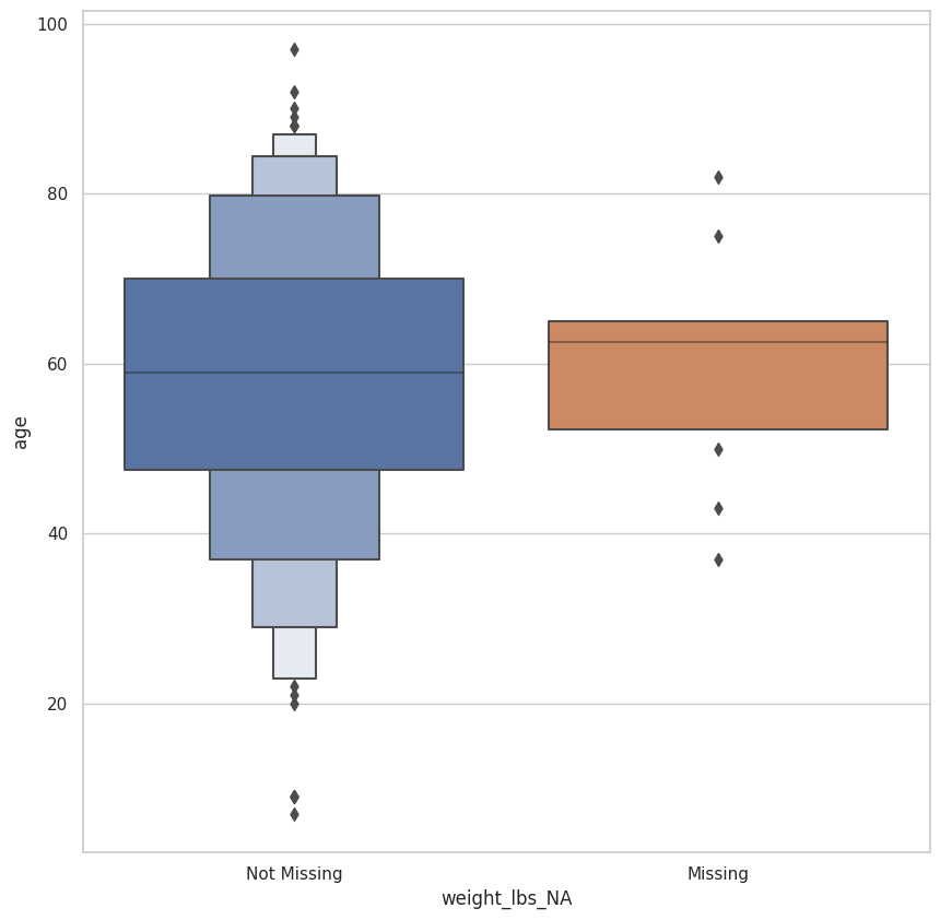
Visualización de valores faltantes en una variable

(
    riskfactors_df
    .missing
    .bind_shadow_matrix(only_missing=True)
    .pipe(
        lambda df:(
            sns.boxenplot(
                data=df,
                x="weight_lbs_NA",
                y="age"
            )
        )
    )
)

<AxesSubplot:xlabel='weight_lbs_NA', ylabel='age'>

(
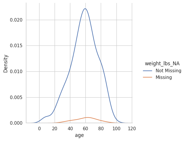
    riskfactors_df
    .missing
    .bind_shadow_matrix(only_missing=True)
    .pipe(
        lambda df:(
            sns.displot(
                data=df,
                x="age",
                hue="weight_lbs_NA",
                kind="kde"
            )
        )
    )
)

<seaborn.axisgrid.FacetGrid at 0x7f3f7c0a0670>

(
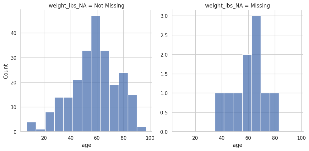
    riskfactors_df
    .missing
    .bind_shadow_matrix(only_missing=True)
    .pipe(
        lambda df:(
            sns.displot(
                data=df,
                x="age",
                col="weight_lbs_NA",
                facet_kws={
                    "sharey":False
                }
            )
        )
    )
)

<seaborn.axisgrid.FacetGrid at 0x7f3f7c121c70>

(
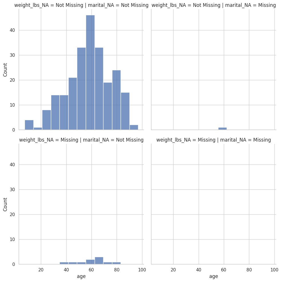
    riskfactors_df
    .missing
    .bind_shadow_matrix(only_missing=True)
    .pipe(
        lambda df:(
            sns.displot(
                data=df,
                x="age",
                col="marital_NA",
                row="weight_lbs_NA"
            )
        )
    )
)

<seaborn.axisgrid.FacetGrid at 0x7f3f755a59a0>

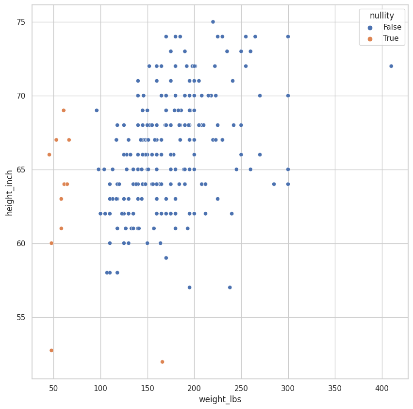
Visualización de valores faltantes en dos variables

def column_fill_with_dummies(
    column: pd.Series,
    proportion_below: float=0.10,
    jitter: float=0.075,
    seed: int=42
) -> pd.Series:

    column = column.copy(deep=True)

    # Extract values metadata
    missing_mask = column.isna()
    number_missing_values = missing_mask.sum()
    column_range = column.max() - column.min()

    # Shift data
    column_shift = column.min() - column.min() * proportion_below

    # Create the "jitter" (noise) to be added around the points.
    np.random.seed(seed)
    column_jitter = (np.random.rand(number_missing_values) - 2) * column_range * jitter

    # Save new dummy data.
    column[missing_mask] = column_shift + column_jitter

    return column

(
    riskfactors_df
    .select_dtypes(
        exclude="category"
    )
    .pipe(
        lambda df: df[df.columns[df.isna().any()]]
    )
    .missing.bind_shadow_matrix(true_string = True, false_string = False)
    .apply(
        lambda column: column if "_NA" in column.name else column_fill_with_dummies(column, proportion_below=0.05, jitter = 0.075)
    )
    .assign(
        nullity = lambda df: df.weight_lbs_NA | df.height_inch_NA
    )
    .pipe(
        lambda df: (
            sns.scatterplot(
                data = df,
                x = "weight_lbs",
                y = "height_inch",
                hue = "nullity"
            )
        )
    )
)

<AxesSubplot:xlabel='weight_lbs', ylabel='height_inch'>

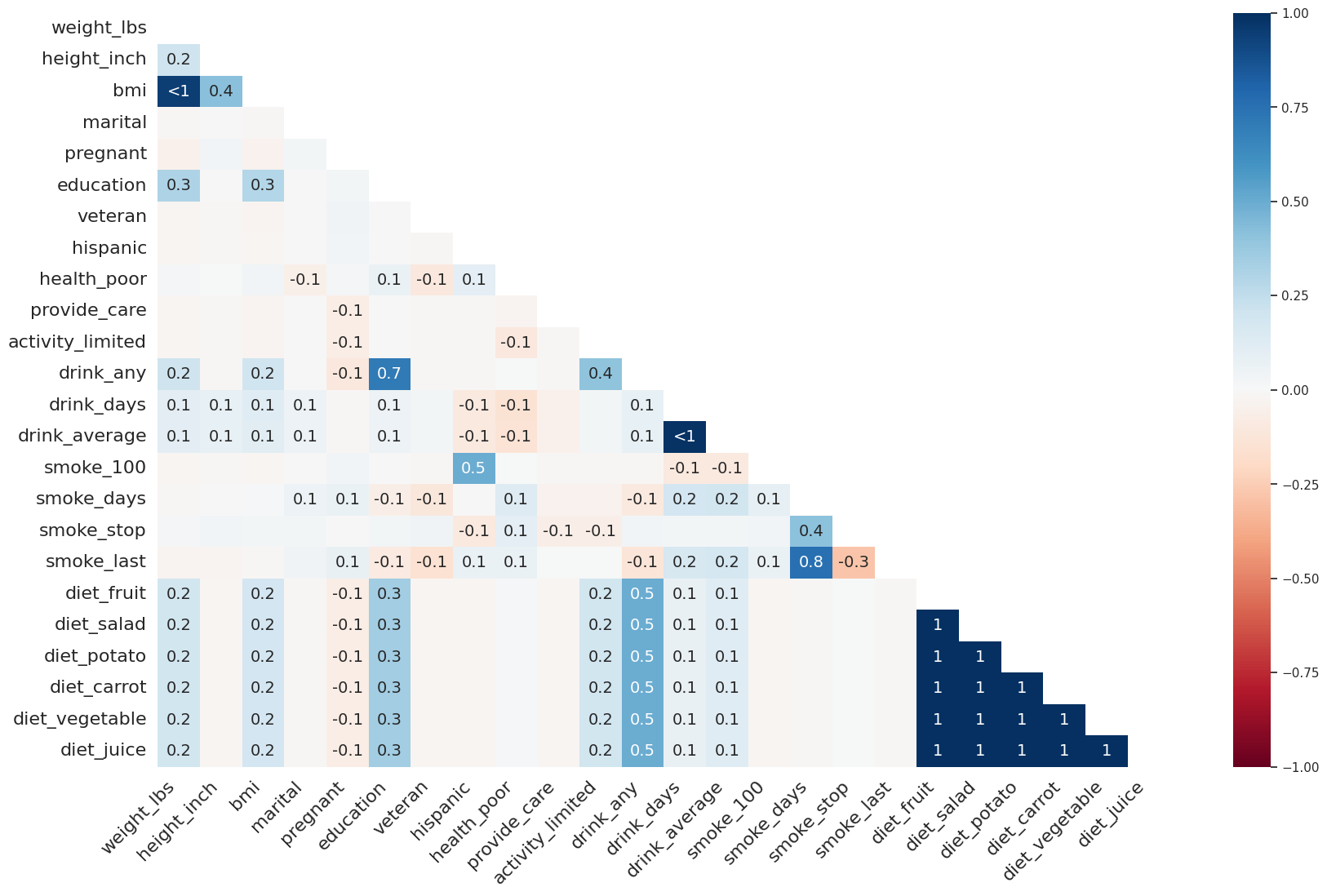
Correlación de nulidad

missingno.heatmap(
    df=riskfactors_df
)

/shared-libs/python3.9/py/lib/python3.9/site-packages/seaborn/matrix.py:306: MatplotlibDeprecationWarning: Auto-removal of grids by pcolor() and pcolormesh() is deprecated since 3.5 and will be removed two minor releases later; please call grid(False) first.
  mesh = ax.pcolormesh(self.plot_data, cmap=self.cmap, **kws)
/shared-libs/python3.9/py/lib/python3.9/site-packages/seaborn/matrix.py:316: MatplotlibDeprecationWarning: Auto-removal of grids by pcolor() and pcolormesh() is deprecated since 3.5 and will be removed two minor releases later; please call grid(False) first.
  cb = ax.figure.colorbar(mesh, cax, ax, **self.cbar_kws)

<AxesSubplot:>

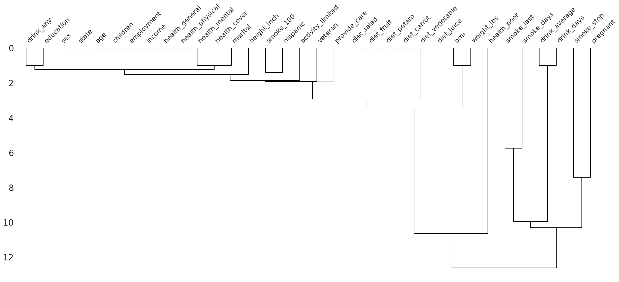
missingno.dendrogram(
    df=riskfactors_df
)

/root/venv/lib/python3.9/site-packages/missingno/missingno.py:475: MatplotlibDeprecationWarning: The 'b' parameter of grid() has been renamed 'visible' since Matplotlib 3.5; support for the old name will be dropped two minor releases later.
  ax0.grid(b=False)

<AxesSubplot:>

Eliminación de valores faltantes

🚧 Advertencia

La eliminación de valores faltantes asume que los valores faltantes están perdidos completamente al azar (MCAR). En cualquier otro caso, realizar una eliminación de valores faltantes podrá ocasionar sesgos en los análisis y modelos subsecuentes.

Primero observa el número total de observaciones y variables que tiene tu conjunto de datos.

riskfactors_df.shape

(245, 34)

Pairwise deletion (eliminación por pares)

Esto consiste en ignorar valores nulos para realziar operaciones como calculos de promedio, conteos, etc

riskfactors_df.weight_lbs.size, riskfactors_df.weight_lbs.count()

(245, 235)

En este caso, en size se cuentan todos los datos. Mientras que en count() solo se cuentan los datos no nulos

Listwise Deletion or Complete Case (Eliminación por lista o caso completo)

Este procedimiento consiste en borrar todo el registro (o fila) si es que hay un valor faltante

Con base en 1 columna

(
    riskfactors_df
    .dropna(
        subset=["weight_lbs"],
        how="any"
    )
)

	state	sex	age	weight_lbs	height_inch	bmi	marital	pregnant	children	education	...	smoke_100	smoke_days	smoke_stop	smoke_last	diet_fruit	diet_salad	diet_potato	diet_carrot	diet_vegetable	diet_juice
0	26	Female	49	190	64	32.68	Married	NaN	0	6	...	No	NaN	NaN	NaN	1095	261	104	156	521	12
1	40	Female	48	170	68	25.90	Divorced	NaN	0	5	...	No	NaN	NaN	NaN	52	209	52	0	52	0
2	72	Female	55	163	64	28.04	Married	NaN	0	4	...	No	NaN	NaN	NaN	36	156	52	24	24	24
3	42	Male	42	230	74	29.59	Married	NaN	1	6	...	No	NaN	NaN	NaN	NaN	NaN	NaN	NaN	NaN	NaN
4	32	Female	66	135	62	24.74	Widowed	NaN	0	5	...	Yes	Everyday	Yes	NaN	-7	261	209	261	365	104
...	...	...	...	...	...	...	...	...	...	...	...	...	...	...	...	...	...	...	...	...	...
240	10	Female	79	144	63	25.56	Widowed	NaN	0	4	...	No	NaN	NaN	NaN	-7	-7	-7	-7	-7	-7
241	46	Male	45	170	74	21.87	Divorced	NaN	2	4	...	No	NaN	NaN	NaN	52	52	52	24	52	24
242	15	Male	62	175	71	24.46	Divorced	NaN	0	6	...	Yes	Not@All	NaN	7	365	156	104	52	730	365
243	34	Female	62	138	64	23.74	Married	NaN	0	4	...	Yes	Everyday	No	NaN	730	0	24	156	104	0
244	18	Male	9	200	70	28.76	Married	NaN	0	4	...	Yes	Not@All	NaN	7	52	104	52	0	104	104

235 rows × 34 columns

Se borraron los registros si weight_lbs esta faltando

Con base en 2 o más columnas

(
    riskfactors_df
    .dropna(
        subset=["weight_lbs", "height_inch"],
        how="any"
    )
)

	state	sex	age	weight_lbs	height_inch	bmi	marital	pregnant	children	education	...	smoke_100	smoke_days	smoke_stop	smoke_last	diet_fruit	diet_salad	diet_potato	diet_carrot	diet_vegetable	diet_juice
0	26	Female	49	190	64	32.68	Married	NaN	0	6	...	No	NaN	NaN	NaN	1095	261	104	156	521	12
1	40	Female	48	170	68	25.90	Divorced	NaN	0	5	...	No	NaN	NaN	NaN	52	209	52	0	52	0
2	72	Female	55	163	64	28.04	Married	NaN	0	4	...	No	NaN	NaN	NaN	36	156	52	24	24	24
3	42	Male	42	230	74	29.59	Married	NaN	1	6	...	No	NaN	NaN	NaN	NaN	NaN	NaN	NaN	NaN	NaN
4	32	Female	66	135	62	24.74	Widowed	NaN	0	5	...	Yes	Everyday	Yes	NaN	-7	261	209	261	365	104
...	...	...	...	...	...	...	...	...	...	...	...	...	...	...	...	...	...	...	...	...	...
240	10	Female	79	144	63	25.56	Widowed	NaN	0	4	...	No	NaN	NaN	NaN	-7	-7	-7	-7	-7	-7
241	46	Male	45	170	74	21.87	Divorced	NaN	2	4	...	No	NaN	NaN	NaN	52	52	52	24	52	24
242	15	Male	62	175	71	24.46	Divorced	NaN	0	6	...	Yes	Not@All	NaN	7	365	156	104	52	730	365
243	34	Female	62	138	64	23.74	Married	NaN	0	4	...	Yes	Everyday	No	NaN	730	0	24	156	104	0
244	18	Male	9	200	70	28.76	Married	NaN	0	4	...	Yes	Not@All	NaN	7	52	104	52	0	104	104

234 rows × 34 columns

Se borraron los registros si weight_lbs y height_inch estan faltando

(
    riskfactors_df
    .dropna(
        subset=["weight_lbs", "height_inch"],
        how="all"
    )
)

	state	sex	age	weight_lbs	height_inch	bmi	marital	pregnant	children	education	...	smoke_100	smoke_days	smoke_stop	smoke_last	diet_fruit	diet_salad	diet_potato	diet_carrot	diet_vegetable	diet_juice
0	26	Female	49	190	64	32.68	Married	NaN	0	6	...	No	NaN	NaN	NaN	1095	261	104	156	521	12
1	40	Female	48	170	68	25.90	Divorced	NaN	0	5	...	No	NaN	NaN	NaN	52	209	52	0	52	0
2	72	Female	55	163	64	28.04	Married	NaN	0	4	...	No	NaN	NaN	NaN	36	156	52	24	24	24
3	42	Male	42	230	74	29.59	Married	NaN	1	6	...	No	NaN	NaN	NaN	NaN	NaN	NaN	NaN	NaN	NaN
4	32	Female	66	135	62	24.74	Widowed	NaN	0	5	...	Yes	Everyday	Yes	NaN	-7	261	209	261	365	104
...	...	...	...	...	...	...	...	...	...	...	...	...	...	...	...	...	...	...	...	...	...
240	10	Female	79	144	63	25.56	Widowed	NaN	0	4	...	No	NaN	NaN	NaN	-7	-7	-7	-7	-7	-7
241	46	Male	45	170	74	21.87	Divorced	NaN	2	4	...	No	NaN	NaN	NaN	52	52	52	24	52	24
242	15	Male	62	175	71	24.46	Divorced	NaN	0	6	...	Yes	Not@All	NaN	7	365	156	104	52	730	365
243	34	Female	62	138	64	23.74	Married	NaN	0	4	...	Yes	Everyday	No	NaN	730	0	24	156	104	0
244	18	Male	9	200	70	28.76	Married	NaN	0	4	...	Yes	Not@All	NaN	7	52	104	52	0	104	104

244 rows × 34 columns

Se borraron los registros si weight_lbs o height_inch estan faltando

Representación gráfica tras la eliminación de los valores faltantes

(
    riskfactors_df
    .dropna(
        subset=["weight_lbs", "height_inch"],
        how="any"
    )
    .select_columns(["weight_lbs", "height_inch"])
    .pipe(missingno.matrix)
)

/root/venv/lib/python3.9/site-packages/missingno/missingno.py:73: MatplotlibDeprecationWarning: The 'b' parameter of grid() has been renamed 'visible' since Matplotlib 3.5; support for the old name will be dropped two minor releases later.
  ax0.grid(b=False)
/root/venv/lib/python3.9/site-packages/missingno/missingno.py:142: MatplotlibDeprecationWarning: The 'b' parameter of grid() has been renamed 'visible' since Matplotlib 3.5; support for the old name will be dropped two minor releases later.
  ax1.grid(b=False)

<AxesSubplot:>

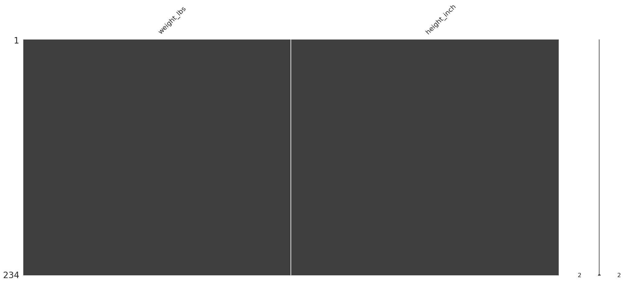
Se confirma en el grafico que no faltan datos

Imputación básica de valores faltantes

Imputacion es reemplazar los datos faltantes por datos con sentido, puedes basarte en:

• algun estadistico que venga de los datos

• un valor por contexto

• un valor extraido de un modelo de machine learning

Imputación con base en el contexto

implicit_to_explicit_df = pd.DataFrame(
    data={
        "name": ["lynn", np.nan, "zelda", np.nan, "shadowsong", np.nan],
        "time": ["morning", "afternoon", "morning", "afternoon", "morning", "afternoon",],
        "value": [350, 310, 320, 350, 310, 320]
    }
)

implicit_to_explicit_df

	name	time	value
0	lynn	morning	350
1	NaN	afternoon	310
2	zelda	morning	320
3	NaN	afternoon	350
4	shadowsong	morning	310
5	NaN	afternoon	320

En este caso, es obvio que hay que poner el mismo nombre de la fila previa en el valor faltante, eso es contexto.

Como se rellena de manera rapida?

implicit_to_explicit_df.ffill()

	name	time	value
0	lynn	morning	350
1	lynn	afternoon	310
2	zelda	morning	320
3	zelda	afternoon	350
4	shadowsong	morning	310
5	shadowsong	afternoon	320

Imputación de un único valor

(
    riskfactors_df
    .select_columns("weight_lbs", "height_inch", "bmi")
    .missing.bind_shadow_matrix(true_string = True, false_string = False)
    .apply(
        axis = "rows",
        func = lambda column : column.fillna(column.mean()) if "_NA" not in column.name else column
        # Basicamente se acaba de llenar el valor faltante con el promedio de su respectiva columna
    )
)

	weight_lbs	height_inch	bmi	weight_lbs_NA	height_inch_NA	bmi_NA
0	190.0	64.0	32.68	False	False	False
1	170.0	68.0	25.90	False	False	False
2	163.0	64.0	28.04	False	False	False
3	230.0	74.0	29.59	False	False	False
4	135.0	62.0	24.74	False	False	False
...	...	...	...	...	...	...
240	144.0	63.0	25.56	False	False	False
241	170.0	74.0	21.87	False	False	False
242	175.0	71.0	24.46	False	False	False
243	138.0	64.0	23.74	False	False	False
244	200.0	70.0	28.76	False	False	False

245 rows × 6 columns

Basicamente se acaba de llenar el valor faltante con el promedio de su respectiva columna

visualizando ese procedimiento:

(
    riskfactors_df
    .select_columns("weight_lbs", "height_inch", "bmi")
    .missing.bind_shadow_matrix(true_string = True, false_string = False)
    .apply(
        axis = "rows",
        func = lambda column : column.fillna(column.mean()) if "_NA" not in column.name else column
        # Basicamente se acaba de llenar el valor faltante con el promedio de su respectiva columna
    )
    .pipe(
        lambda df: (
            sns.displot(
                data=df,
                x="weight_lbs",
                hue="weight_lbs_NA"
            )
        )
    )
)

<seaborn.axisgrid.FacetGrid at 0x7f3faf6c0ca0>

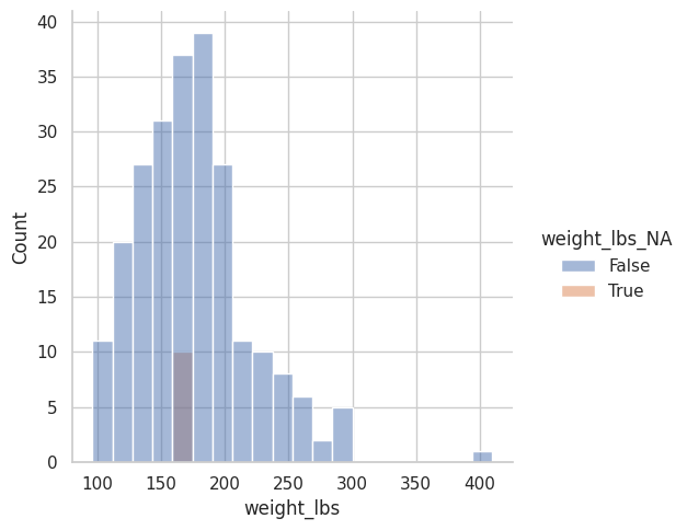
Se confirma que los valores faltantes ahora corresponden al promedio.

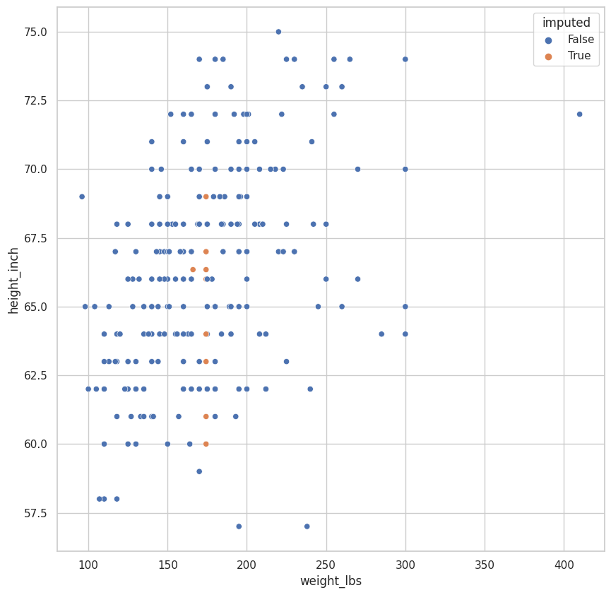
Scatterplot con valores imputados

(
    riskfactors_df
    .select_columns("weight_lbs", "height_inch", "bmi")
    .missing.bind_shadow_matrix(true_string = True, false_string = False)
    .apply(
        axis = "rows",
        func = lambda column : column.fillna(column.mean()) if "_NA" not in column.name else column
    )
    .assign(
        imputed=lambda df: df.weight_lbs_NA | df.height_inch_NA
    )
    .pipe(
        lambda df: (
            sns.scatterplot(
                data=df,
                x="weight_lbs",
                y="height_inch",
                hue="imputed"
            )
        )
    )
)

<AxesSubplot:xlabel='weight_lbs', ylabel='height_inch'>

(
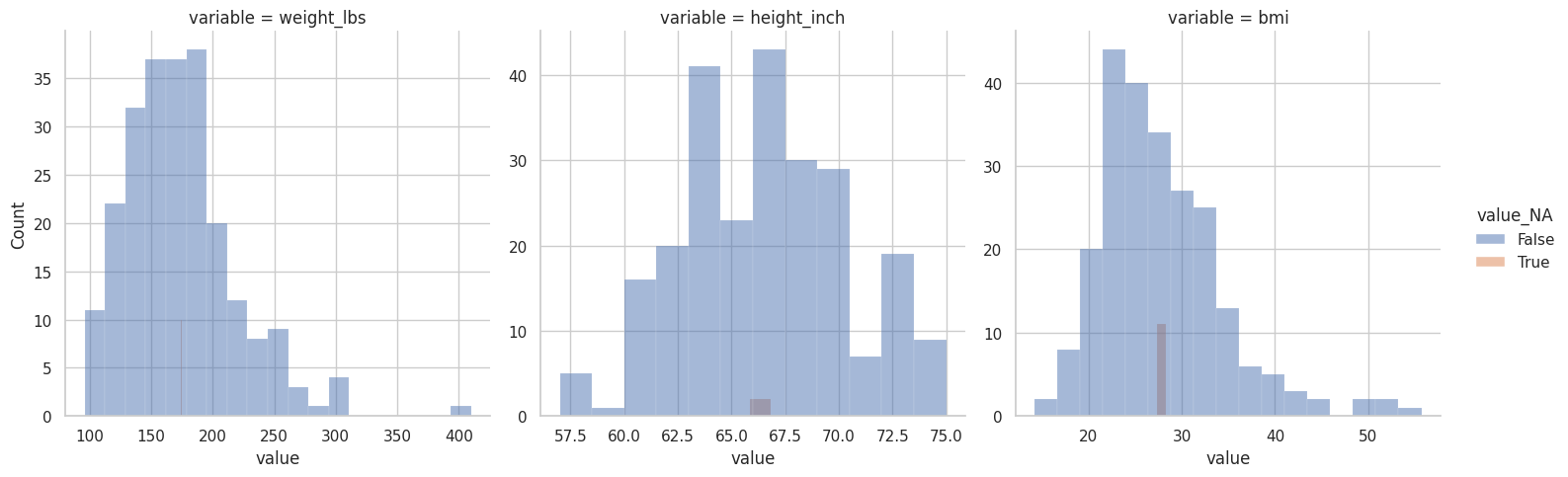
    riskfactors_df
    .select_columns("weight_lbs", "height_inch", "bmi")
    .missing.bind_shadow_matrix(true_string = True, false_string = False)
    .apply(
        axis = "rows",
        func = lambda column : column.fillna(column.mean()) if "_NA" not in column.name else column
    )
    .pivot_longer(
        index="*_NA"
    )
    .pivot_longer(
        index=["variable", "value"],
        names_to = "variable_NA",
        values_to = "value_NA"
    )
    .assign(
        valid=lambda df:df.apply(axis="columns", func = lambda column: column.variable in column.variable_NA)
    )
    .query("valid")
    .pipe(
        lambda df: (
            sns.displot(
                data=df,
                x="value",
                hue="value_NA",
                col="variable",
                common_bins=False,
                facet_kws={
                    "sharex": False,
                    "sharey": False
                }
            )
        )
    )
)

<seaborn.axisgrid.FacetGrid at 0x7f3fbf26bd60>

Created in Deepnote