Manejo de Datos Faltantes: Imputación

Configuración de ambiente de trabajo

pip install -r requirements.txt

^C
Requirement already satisfied: pip in c:\users\admin\miniconda3\lib\site-packages (from -r requirements.txt (line 1)) (23.1.2)
Collecting pyjanitor (from -r requirements.txt (line 2))
  Using cached pyjanitor-0.25.0-py3-none-any.whl (171 kB)
Requirement already satisfied: matplotlib in c:\users\admin\miniconda3\lib\site-packages (from -r requirements.txt (line 3)) (3.7.2)
Collecting missingno (from -r requirements.txt (line 4))
  Using cached missingno-0.5.2-py3-none-any.whl (8.7 kB)
Requirement already satisfied: numpy in c:\users\admin\miniconda3\lib\site-packages (from -r requirements.txt (line 5)) (1.25.2)
Requirement already satisfied: pandas in c:\users\admin\miniconda3\lib\site-packages (from -r requirements.txt (line 6)) (2.1.0)
Requirement already satisfied: pandas-flavor in c:\users\admin\miniconda3\lib\site-packages (from -r requirements.txt (line 7)) (0.6.0)
Collecting pandas-profiling (from -r requirements.txt (line 8))
  Using cached pandas_profiling-3.2.0-py2.py3-none-any.whl (262 kB)
Requirement already satisfied: seaborn in c:\users\admin\miniconda3\lib\site-packages (from -r requirements.txt (line 9)) (0.12.2)
Collecting session-info (from -r requirements.txt (line 10))
  Using cached session_info-1.0.0.tar.gz (24 kB)
  Preparing metadata (setup.py): started
  Preparing metadata (setup.py): finished with status 'done'
Collecting ipywidgets (from -r requirements.txt (line 11))
  Using cached ipywidgets-8.1.0-py3-none-any.whl (139 kB)
Collecting ozon3 (from -r requirements.txt (line 12))
  Using cached ozon3-4.0.2-py3-none-any.whl (27 kB)
Collecting pyreadr (from -r requirements.txt (line 13))
  Using cached pyreadr-0.4.9-cp311-cp311-win_amd64.whl (1.3 MB)
Collecting upsetplot (from -r requirements.txt (line 14))
  Using cached UpSetPlot-0.8.0.tar.gz (22 kB)
  Preparing metadata (setup.py): started
  Preparing metadata (setup.py): finished with status 'done'
Collecting statsmodels==0.13.2 (from -r requirements.txt (line 15))
  Using cached statsmodels-0.13.2.tar.gz (17.9 MB)
  Installing build dependencies: started

Note: you may need to restart the kernel to use updated packages.

Importar librerías

import janitor
import matplotlib.pyplot as plt
import missingno
import nhanes.load
import numpy as np
import pandas as pd
import scipy.stats
import seaborn as sns
import session_info
import sklearn.compose
import sklearn.impute
import sklearn.preprocessing
import statsmodels.api as sm
import statsmodels.datasets
import statsmodels.formula.api as smf

from sklearn.ensemble import RandomForestRegressor
from sklearn.experimental import enable_iterative_imputer
from sklearn.kernel_approximation import Nystroem
from sklearn.linear_model import BayesianRidge, Ridge
from sklearn.neighbors import KNeighborsRegressor
from statsmodels.graphics.mosaicplot import mosaic

Importar funciones personalizadas

%run pandas-missing-extension.ipynb

/root/venv/lib/python3.9/site-packages/upsetplot/plotting.py:20: MatplotlibDeprecationWarning: The matplotlib.tight_layout module was deprecated in Matplotlib 3.6 and will be removed two minor releases later.
  from matplotlib.tight_layout import get_renderer

Configurar el aspecto general de las gráficas del proyecto

%matplotlib inline

sns.set(
    rc={
        "figure.figsize": (8, 6)
    }
)

sns.set_style("whitegrid")

El problema de trabajar con valores faltantes

airquality_df = (
    sm.datasets.get_rdataset("airquality")
    .data
    .clean_names(
        case_type = "snake"
    )
    .add_column("year", 1973)
    .assign(
        date = lambda df: pd.to_datetime(df[["year", "month", "day"]])
    )
    .sort_values(by = "date")
    .set_index("date")
)

airquality_df

	ozone	solar_r	wind	temp	month	day	year
date
1973-05-01	41.0	190.0	7.4	67	5	1	1973
1973-05-02	36.0	118.0	8.0	72	5	2	1973
1973-05-03	12.0	149.0	12.6	74	5	3	1973
1973-05-04	18.0	313.0	11.5	62	5	4	1973
1973-05-05	NaN	NaN	14.3	56	5	5	1973
...	...	...	...	...	...	...	...
1973-09-26	30.0	193.0	6.9	70	9	26	1973
1973-09-27	NaN	145.0	13.2	77	9	27	1973
1973-09-28	14.0	191.0	14.3	75	9	28	1973
1973-09-29	18.0	131.0	8.0	76	9	29	1973
1973-09-30	20.0	223.0	11.5	68	9	30	1973

153 rows × 7 columns

Hagamos dos modelos de regresion para predecir la temperatura en funcion de otras variables:

(
    smf.ols(
        formula = "temp ~ ozone",
        data = airquality_df
    )
    .fit()
    .summary()
    .tables[0]
)

OLS Regression Results

Dep. Variable:	temp	R-squared:	0.488
Model:	OLS	Adj. R-squared:	0.483
Method:	Least Squares	F-statistic:	108.5
Date:	Wed, 25 Jan 2023	Prob (F-statistic):	2.93e-18
Time:	03:02:38	Log-Likelihood:	-386.27
No. Observations:	116	AIC:	776.5
Df Residuals:	114	BIC:	782.1
Df Model:	1
Covariance Type:	nonrobust

(
    smf.ols(
        formula = "temp ~ ozone + solar_r",
        data = airquality_df
    )
    .fit()
    .summary()
    .tables[0]
)

OLS Regression Results

Dep. Variable:	temp	R-squared:	0.491
Model:	OLS	Adj. R-squared:	0.481
Method:	Least Squares	F-statistic:	52.07
Date:	Wed, 25 Jan 2023	Prob (F-statistic):	1.47e-16
Time:	03:02:38	Log-Likelihood:	-369.78
No. Observations:	111	AIC:	745.6
Df Residuals:	108	BIC:	753.7
Df Model:	2
Covariance Type:	nonrobust

Si analizas el numero de observaciones, veras que un modelo ignora cierta cantidad de valores faltantes mientras que el otro no lo hace. No es recomendable en este caso usar el R^2 para comparar ambos modelos como equivalentes. Por lo tanto toca imputar datos y asi poder realizarlo

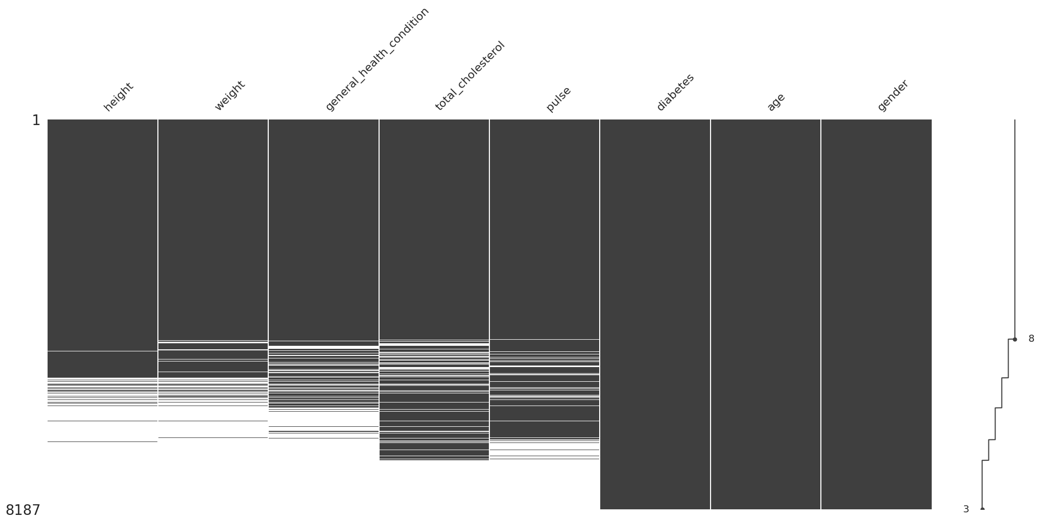
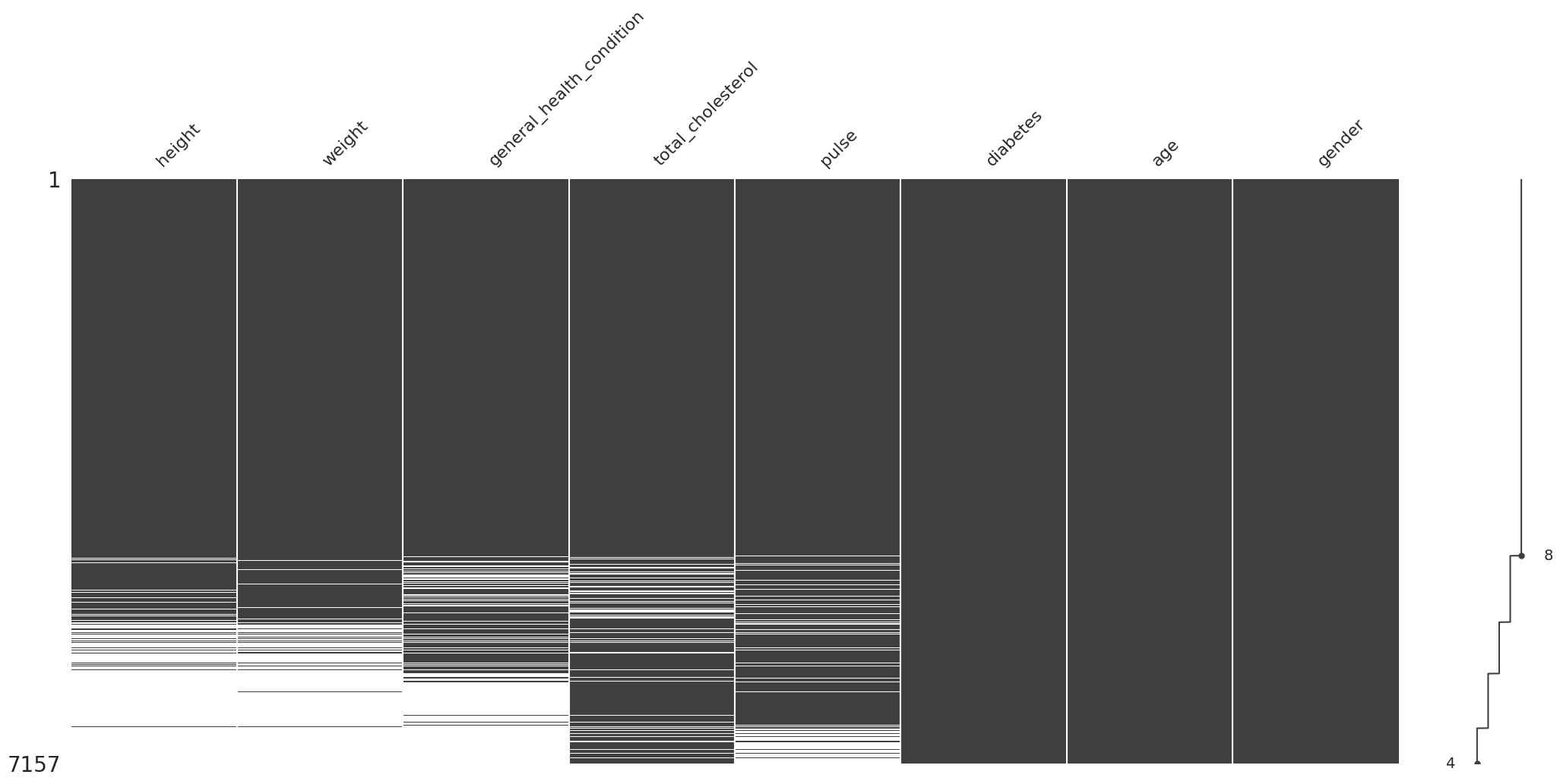
Preparando datos: National Health and Nutrition Examination Survey

%run download-data-and-load-it.ipynb

/root/venv/lib/python3.9/site-packages/missingno/missingno.py:73: MatplotlibDeprecationWarning: The 'b' parameter of grid() has been renamed 'visible' since Matplotlib 3.5; support for the old name will be dropped two minor releases later.
  ax0.grid(b=False)
/root/venv/lib/python3.9/site-packages/missingno/missingno.py:142: MatplotlibDeprecationWarning: The 'b' parameter of grid() has been renamed 'visible' since Matplotlib 3.5; support for the old name will be dropped two minor releases later.
  ax1.grid(b=False)

/root/venv/lib/python3.9/site-packages/missingno/missingno.py:73: MatplotlibDeprecationWarning: The 'b' parameter of grid() has been renamed 'visible' since Matplotlib 3.5; support for the old name will be dropped two minor releases later.
  ax0.grid(b=False)
/root/venv/lib/python3.9/site-packages/missingno/missingno.py:142: MatplotlibDeprecationWarning: The 'b' parameter of grid() has been renamed 'visible' since Matplotlib 3.5; support for the old name will be dropped two minor releases later.
  ax1.grid(b=False)

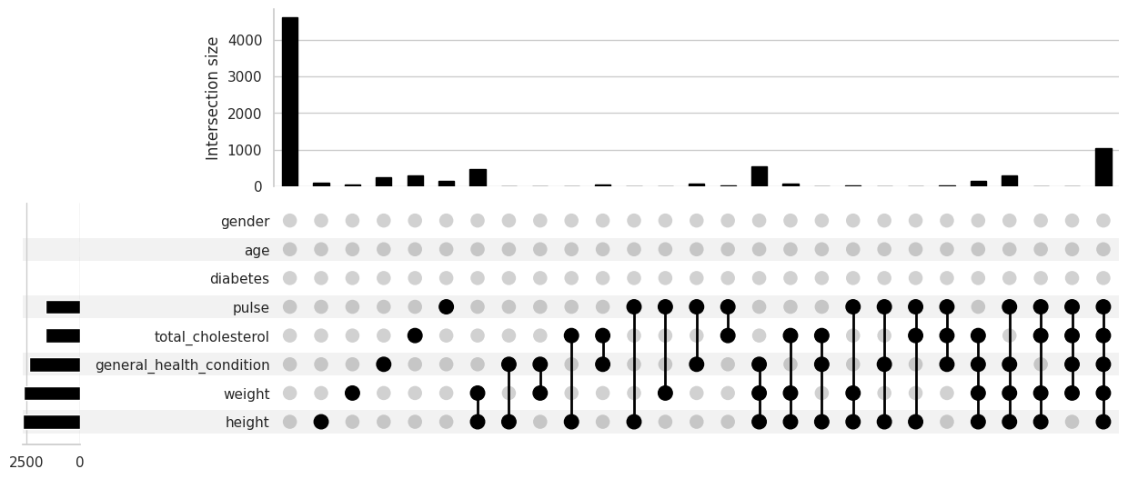
Consideración y evaluación de los distintos tipos de valores faltantes

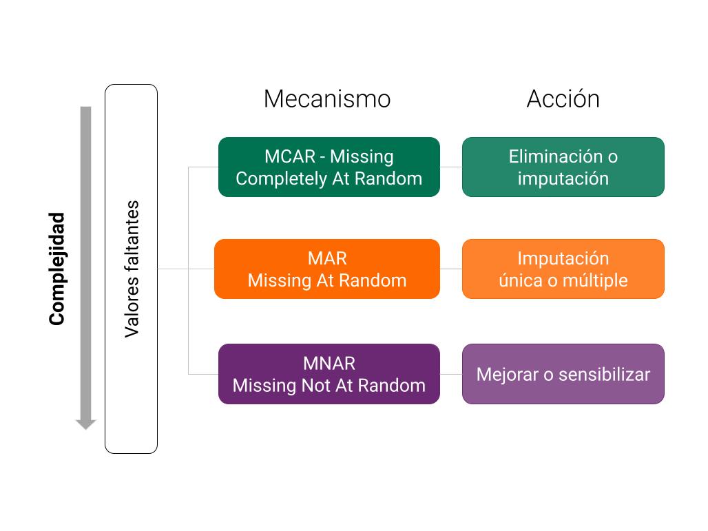
Evaluación del mecanismo de valores faltantes por prueba de t-test

📘 Información

two-sided: las medias de las distribuciones subyacentes a las muestras son desiguales.
less: la media de la distribución subyacente a la primera muestra es menor que la media de la distribución subyacente a la segunda muestra.
greater: la media de la distribución subyacente a la primera muestra es mayor que la media de la distribución subyacente a la segunda muestra.

female_weight, male_weight = (
    nhanes_df
    .select_columns("gender", "weight")
    .transform_column(
        "weight",
        lambda x: x.isna(),
        elementwise = False
    )
    .groupby("gender")
    .weight
    .pipe(
        lambda df: (
            df.get_group("Female"),
            df.get_group("Male")
        )
    )
)

# Ahora se hace una prueba estadistica para determinar si hay o no diferencia en la presencia
# o ausencia de valores de peso

scipy.stats.ttest_ind(
    a = female_weight,
    b = male_weight,
    alternative="two-sided"
)

Ttest_indResult(statistic=-0.3621032192538131, pvalue=0.7172855918077239)

Dado que pvalue < 0.05, no se rechaza la hipotesis nula.

No existe diferencia estadistica entre los valores faltantes

Los datos entonces no estan perdidos al azar entre hombres y mujeres

Tratamiento de variables categóricas para imputación de valores faltantes

# Primero se realiza una copia del dataframe original
nhanes_transformed_df = nhanes_df.copy(deep=True)

Codificación ordinal

📘 Información

Una codificación ordinal implica mapear cada etiqueta (categoría) única a un valor entero. A su vez, la codificación ordinal también es conocida como codificación entera.

Ejemplo

Dado un conjunto de datos con dos características, encontraremos los valores únicos por cataracterística y los transformaremos utilizando una codificación ordinal.

encoder = sklearn.preprocessing.OrdinalEncoder()

X = [["Male"], ["Female"], ["Female"]]
X

[['Male'], ['Female'], ['Female']]

encoder.fit_transform(X)

array([[1.],
       [0.],
       [0.]])

encoder.categories_

[array(['Female', 'Male'], dtype=object)]

encoder.inverse_transform([[1], [0], [0]])

array([['Male'],
       ['Female'],
       ['Female']], dtype=object)

Aplicando la codificación ordinal a todas tus variables categóricas

categorical_columns = nhanes_df.select_dtypes(include=[object, "category"]).columns

categorical_transformer = sklearn.compose.make_column_transformer(
    (sklearn.preprocessing.OrdinalEncoder(), categorical_columns),
    remainder="passthrough"
    #aqui le dices que no modifique las variables que no son categoricas
)

nhanes_transformed_df = (
    pd.DataFrame(
        categorical_transformer.fit_transform(nhanes_df),
        columns = categorical_transformer.get_feature_names_out(),
        index = nhanes_df.index
    )
    .rename_columns(
        function = lambda x: x.removeprefix("ordinalencoder__")
    )
    .rename_columns(
        function = lambda x: x.removeprefix("remainder__")
    )
)

nhanes_transformed_df

	general_health_condition	gender	height	weight	total_cholesterol	pulse	diabetes	age
SEQN
93705.0	2.0	0.0	63.0	165.0	157.0	52.0	0.0	66.0
93706.0	4.0	1.0	68.0	145.0	148.0	82.0	0.0	18.0
93707.0	2.0	1.0	NaN	NaN	189.0	100.0	0.0	13.0
93709.0	NaN	0.0	62.0	200.0	176.0	74.0	0.0	75.0
93711.0	4.0	1.0	69.0	142.0	238.0	62.0	0.0	56.0
...	...	...	...	...	...	...	...	...
102949.0	0.0	1.0	72.0	180.0	201.0	96.0	0.0	33.0
102953.0	1.0	1.0	65.0	218.0	182.0	78.0	0.0	42.0
102954.0	2.0	0.0	66.0	150.0	172.0	78.0	0.0	41.0
102955.0	4.0	0.0	NaN	NaN	150.0	74.0	0.0	14.0
102956.0	2.0	1.0	69.0	250.0	163.0	76.0	0.0	38.0

7157 rows × 8 columns

One Hot Encoding

nhanes_transformed_df2 = nhanes_df.copy(deep=True)

pandas.get_dummies() vs skelearn.preprocessing.OneHotEncoder()

pandas.get_dummies()

pandas.get_dummies() tiene desventajas comparado con sklearn.preprocessing.onehotencoder(), estas son:

• No sabe lidiar con valores nulos

• Si no se seleccionan todas las columnas, puede que no se detecten todas las categorias

(
    nhanes_transformed_df2
    .select_columns("general_health_condition")
    .pipe(pd.get_dummies)
)

	general_health_condition_Excellent	general_health_condition_Fair or	general_health_condition_Good	general_health_condition_Poor?	general_health_condition_Very good
SEQN
93705.0	0	0	1	0	0
93706.0	0	0	0	0	1
93707.0	0	0	1	0	0
93709.0	0	0	0	0	0
93711.0	0	0	0	0	1
...	...	...	...	...	...
102949.0	1	0	0	0	0
102953.0	0	1	0	0	0
102954.0	0	0	1	0	0
102955.0	0	0	0	0	1
102956.0	0	0	1	0	0

7157 rows × 5 columns

skelearn.preprocessing.OneHotEncoder()

Esta opcion tiene la ventaja que va a detectar automaticamente todas las categorias

transformer = sklearn.compose.make_column_transformer(
    (sklearn.preprocessing.OrdinalEncoder(), ["gender"]),
    (sklearn.preprocessing.OneHotEncoder(), ["general_health_condition"]),
    remainder="passthrough"
)

nhanes_transformed_df2 = (
    pd.DataFrame(
        transformer.fit_transform(nhanes_df),
        columns = transformer.get_feature_names_out(),
        index = nhanes_df.index
    )
    .rename_columns(
        function = lambda x: x.removeprefix("ordinalencoder__")
    )
    .rename_columns(
        function = lambda x: x.removeprefix("remainder__")
    )
    .rename_columns(
        function = lambda x: x.removeprefix("onehotencoder__")
    )
)

nhanes_transformed_df2

	gender	general_health_condition_Excellent	general_health_condition_Fair or	general_health_condition_Good	general_health_condition_Poor?	general_health_condition_Very good	general_health_condition_nan	height	weight	total_cholesterol	pulse	diabetes	age
SEQN
93705.0	0.0	0.0	0.0	1.0	0.0	0.0	0.0	63.0	165.0	157.0	52.0	0.0	66.0
93706.0	1.0	0.0	0.0	0.0	0.0	1.0	0.0	68.0	145.0	148.0	82.0	0.0	18.0
93707.0	1.0	0.0	0.0	1.0	0.0	0.0	0.0	NaN	NaN	189.0	100.0	0.0	13.0
93709.0	0.0	0.0	0.0	0.0	0.0	0.0	1.0	62.0	200.0	176.0	74.0	0.0	75.0
93711.0	1.0	0.0	0.0	0.0	0.0	1.0	0.0	69.0	142.0	238.0	62.0	0.0	56.0
...	...	...	...	...	...	...	...	...	...	...	...	...	...
102949.0	1.0	1.0	0.0	0.0	0.0	0.0	0.0	72.0	180.0	201.0	96.0	0.0	33.0
102953.0	1.0	0.0	1.0	0.0	0.0	0.0	0.0	65.0	218.0	182.0	78.0	0.0	42.0
102954.0	0.0	0.0	0.0	1.0	0.0	0.0	0.0	66.0	150.0	172.0	78.0	0.0	41.0
102955.0	0.0	0.0	0.0	0.0	0.0	1.0	0.0	NaN	NaN	150.0	74.0	0.0	14.0
102956.0	1.0	0.0	0.0	1.0	0.0	0.0	0.0	69.0	250.0	163.0	76.0	0.0	38.0

7157 rows × 13 columns

(
    transformer
    .named_transformers_
    .get("onehotencoder")
    .categories_
)

[array(['Excellent', 'Fair or', 'Good', 'Poor?', 'Very good', nan],
       dtype=object)]

(
    transformer
    .named_transformers_
    .get("onehotencoder")
    .inverse_transform(
        X = [[0, 0, 1, 0, 0, 0]]
    )
)

array([['Good']], dtype=object)

Tipos de imputación de valores faltantes

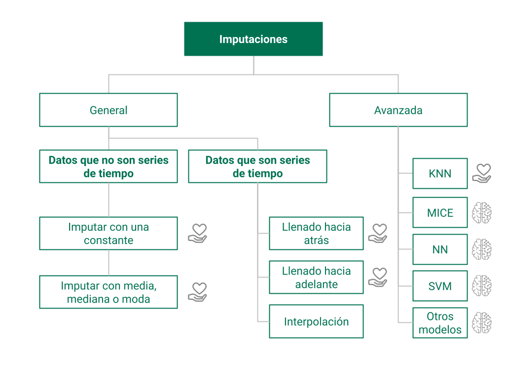
Imputación de un único valor (media, mediana, moda)

Media

(
    nhanes_df
    # janitor
    .transform_column(
        "height",
        lambda x: x.fillna(x.mean()),
        elementwise=False
    )
)

	height	weight	general_health_condition	total_cholesterol	pulse	diabetes	age	gender
SEQN
93705.0	63.00000	165.0	Good	157.0	52.0	0	66.0	Female
93706.0	68.00000	145.0	Very good	148.0	82.0	0	18.0	Male
93707.0	66.25656	NaN	Good	189.0	100.0	0	13.0	Male
93709.0	62.00000	200.0	NaN	176.0	74.0	0	75.0	Female
93711.0	69.00000	142.0	Very good	238.0	62.0	0	56.0	Male
...	...	...	...	...	...	...	...	...
102949.0	72.00000	180.0	Excellent	201.0	96.0	0	33.0	Male
102953.0	65.00000	218.0	Fair or	182.0	78.0	0	42.0	Male
102954.0	66.00000	150.0	Good	172.0	78.0	0	41.0	Female
102955.0	66.25656	NaN	Very good	150.0	74.0	0	14.0	Female
102956.0	69.00000	250.0	Good	163.0	76.0	0	38.0	Male

7157 rows × 8 columns

(
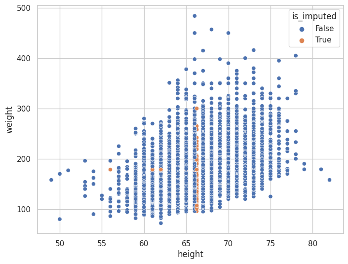
    nhanes_df
    .select_columns("height", "weight")
    .missing.bind_shadow_matrix(True,False, suffix = "_imp")
    .assign(
        height = lambda df: df.height.fillna(value = df.height.mean()),
        weight = lambda df: df.weight.fillna(value = df.weight.mean())
    )
    .missing.scatter_imputation_plot(
        x = "height",
        y = "weight"
    )
)

<AxesSubplot: xlabel='height', ylabel='weight'>

(
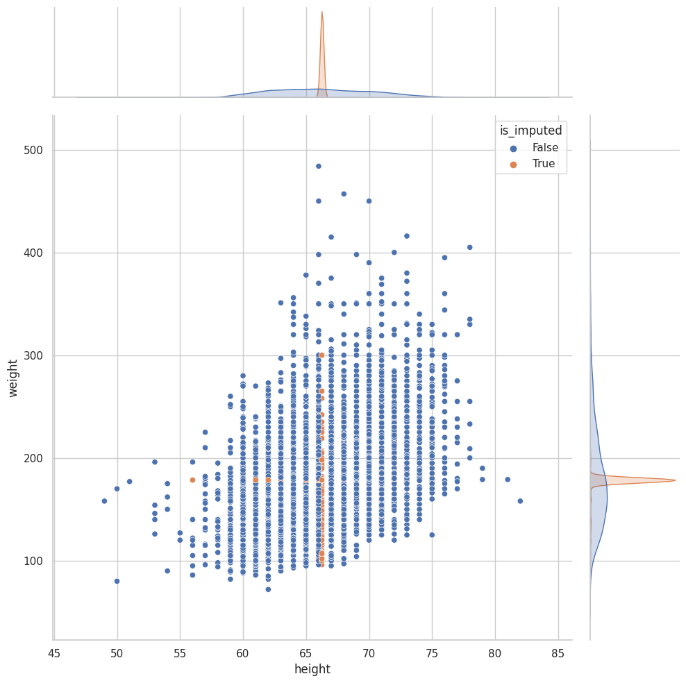
    nhanes_df
    .select_columns("height", "weight")
    .missing.bind_shadow_matrix(True,False, suffix = "_imp")
    .assign(
        height = lambda df: df.height.fillna(value = df.height.mean()),
        weight = lambda df: df.weight.fillna(value = df.weight.mean())
    )
    .missing.scatter_imputation_plot(
        x = "height",
        y = "weight",
        show_marginal= True,
        height = 10
    )
)

<seaborn.axisgrid.JointGrid at 0x7f756fdf28b0>

Imputación por llenado hacia atrás e imputación por llenado hacia adelante

fillna() vs ffill() o bfill()

Forwardfill

Imputa el dato de la fila anterior en nuestro missing value

(
    nhanes_df
    .select_columns("height", "weight")
    
    # .fillna(method = "ffill")
    .ffill()
)

	height	weight
SEQN
93705.0	63.0	165.0
93706.0	68.0	145.0
93707.0	68.0	145.0
93709.0	62.0	200.0
93711.0	69.0	142.0
...	...	...
102949.0	72.0	180.0
102953.0	65.0	218.0
102954.0	66.0	150.0
102955.0	66.0	150.0
102956.0	69.0	250.0

7157 rows × 2 columns

Backfill

Imputa el dato de la fila posterior en nuestro missing value

(
    nhanes_df
    .select_columns("height", "weight")
    
    # .fillna(method = "bfill")
    .bfill()
)

	height	weight
SEQN
93705.0	63.0	165.0
93706.0	68.0	145.0
93707.0	62.0	200.0
93709.0	62.0	200.0
93711.0	69.0	142.0
...	...	...
102949.0	72.0	180.0
102953.0	65.0	218.0
102954.0	66.0	150.0
102955.0	69.0	250.0
102956.0	69.0	250.0

7157 rows × 2 columns

Recomendaciones al imputar valores utilizando ffill() o bfill()

Imputación dentro de dominios e imputación a través de variables correlacionadas

Se recomienda organizar por grupos similares para que no se imputen datos aleatoriamente, sino que el dato que se va a imputar tenga sentido

(
    nhanes_df
    .select_columns("height", "weight", "gender", "diabetes", "general_health_condition")
    .sort_values(
        by = ["gender", "diabetes", "general_health_condition", "height"],
        ascending = True
    )
    .transform_column(
        "weight",
        lambda x: x.ffill(),
        elementwise = False
    )
)

	height	weight	gender	diabetes	general_health_condition
SEQN
94421.0	56.0	115.0	Female	0	Excellent
94187.0	59.0	130.0	Female	0	Excellent
95289.0	59.0	162.0	Female	0	Excellent
97967.0	59.0	130.0	Female	0	Excellent
99125.0	59.0	105.0	Female	0	Excellent
...	...	...	...	...	...
96561.0	74.0	290.0	Male	1	NaN
96954.0	NaN	175.0	Male	1	NaN
97267.0	NaN	175.0	Male	1	NaN
97856.0	NaN	175.0	Male	1	NaN
98317.0	NaN	175.0	Male	1	NaN

7157 rows × 5 columns

(
    nhanes_df
    .select_columns("height", "weight", "gender", "diabetes", "general_health_condition")
    .sort_values(
        by=['gender','diabetes','general_health_condition','weight'],
        ascending=True
    )
    .groupby(["gender", "general_health_condition"], dropna=False)
    .apply(lambda x: x.ffill())
)

/tmp/ipykernel_1384/909901090.py:2: FutureWarning: Not prepending group keys to the result index of transform-like apply. In the future, the group keys will be included in the index, regardless of whether the applied function returns a like-indexed object.
To preserve the previous behavior, use

	>>> .groupby(..., group_keys=False)

To adopt the future behavior and silence this warning, use 

	>>> .groupby(..., group_keys=True)
  nhanes_df

	height	weight	gender	diabetes	general_health_condition
SEQN
94195.0	63.0	90.0	Female	0	Excellent
95793.0	61.0	96.0	Female	0	Excellent
101420.0	59.0	98.0	Female	0	Excellent
94148.0	65.0	100.0	Female	0	Excellent
102062.0	62.0	100.0	Female	0	Excellent
...	...	...	...	...	...
96561.0	74.0	290.0	Male	1	NaN
96869.0	72.0	298.0	Male	1	NaN
97267.0	72.0	298.0	Male	1	NaN
97856.0	72.0	298.0	Male	1	NaN
98317.0	72.0	298.0	Male	1	NaN

7157 rows × 5 columns

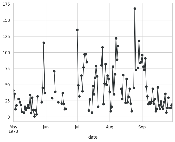
Imputación por interpolación

(
    airquality_df
    .select_columns("ozone")
    .pipe(
        lambda df: (
            df.ozone.plot(color = "#313638", marker= "o")
        )
    )
)

<AxesSubplot: xlabel='date'>

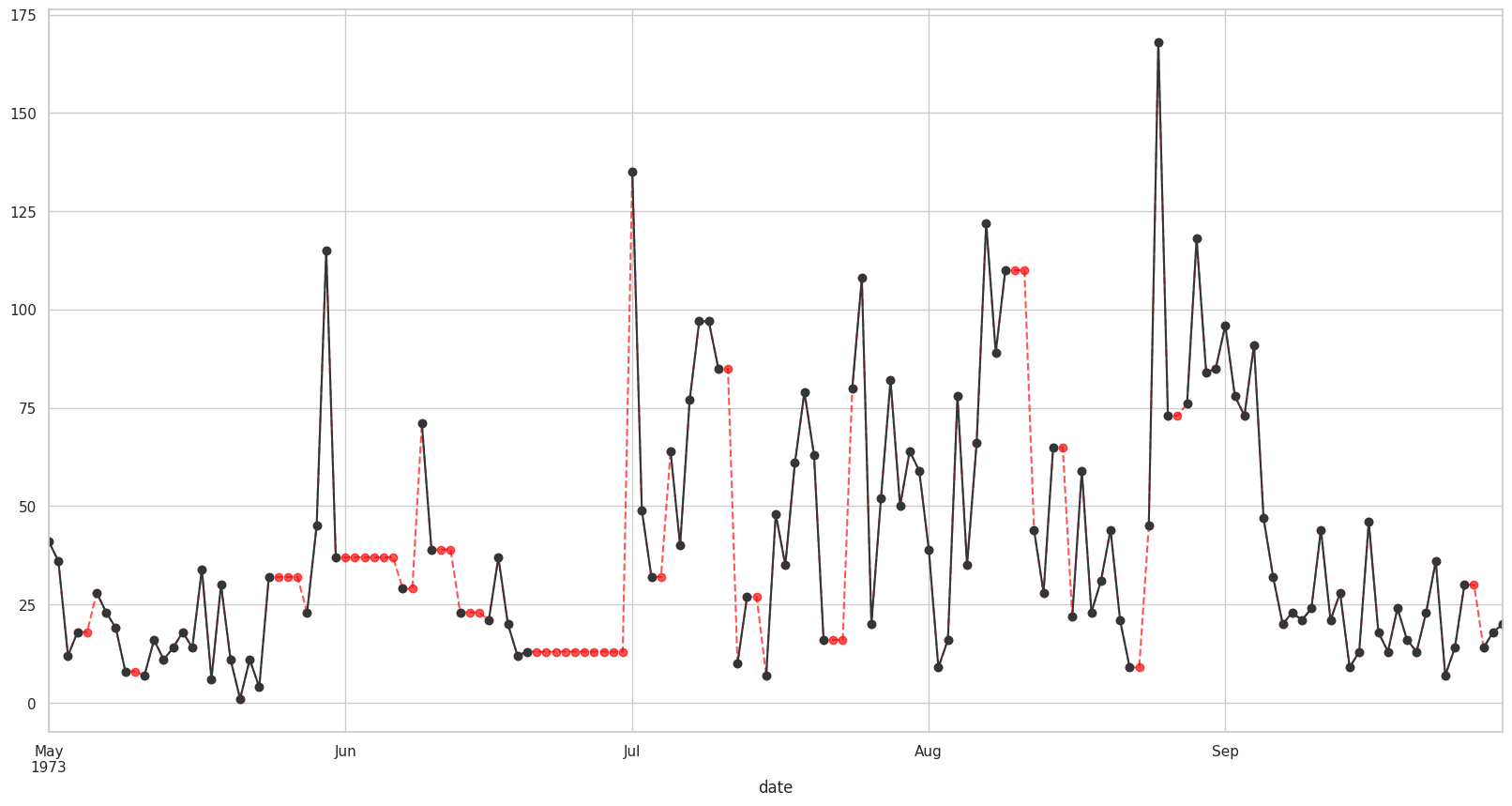
Visualizando con ffill

plt.figure(figsize=(20,10))

(
    airquality_df
    .select_columns("ozone")
    .pipe(
        lambda df: (
            df.ozone.ffill().plot(color= "red", marker="o", alpha=6/9, linestyle="dashed"),
            df.ozone.plot(color = "#313638", marker= "o")
        )
    )
)

(<AxesSubplot: xlabel='date'>, <AxesSubplot: xlabel='date'>)

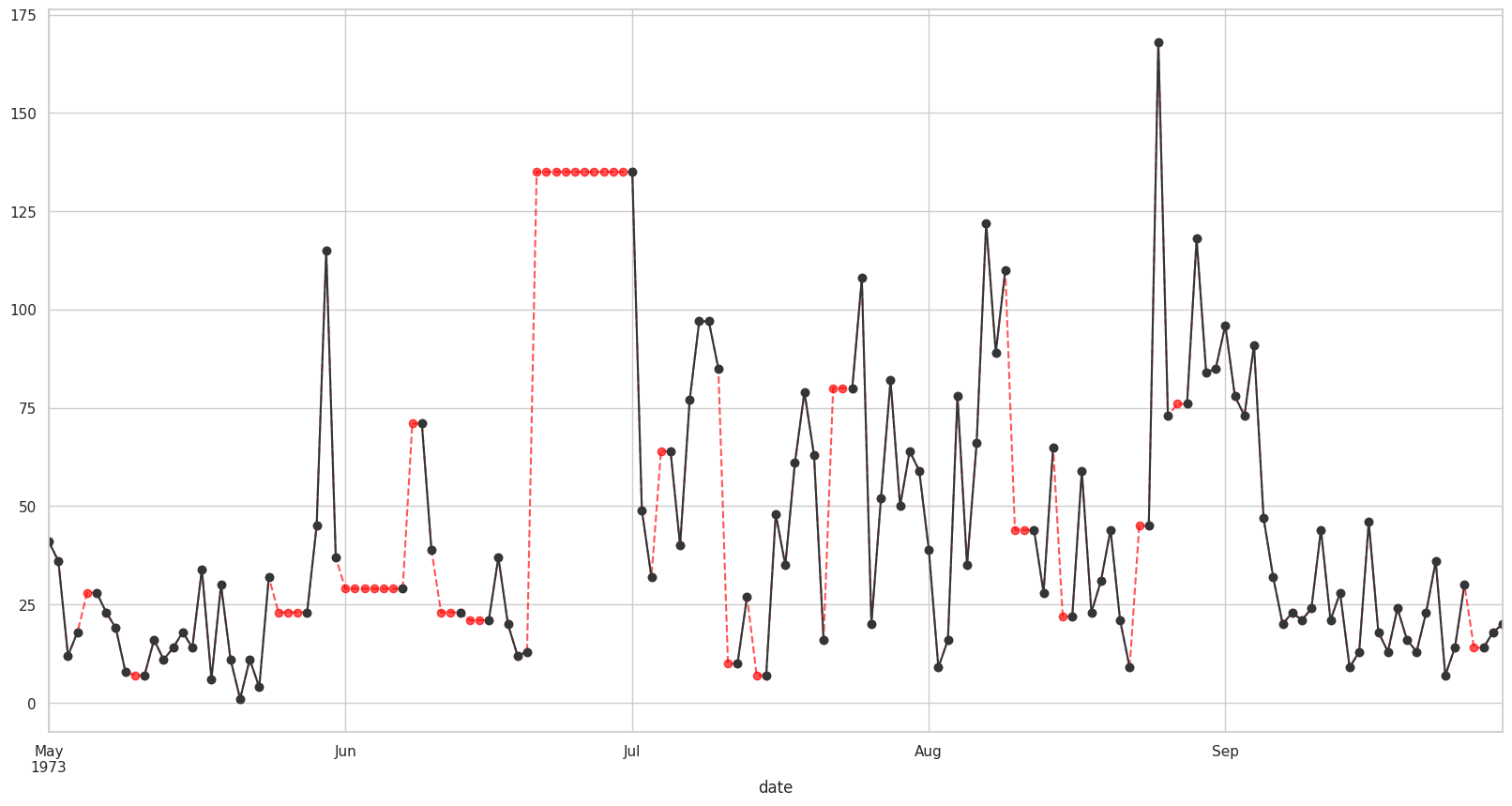
Visualizando con bfill

plt.figure(figsize=(20,10))

(
    airquality_df
    .select_columns("ozone")
    .pipe(
        lambda df: (
            df.ozone.bfill().plot(color= "red", marker="o", alpha=6/9, linestyle="dashed"),
            df.ozone.plot(color = "#313638", marker= "o")
        )
    )
)

(<AxesSubplot: xlabel='date'>, <AxesSubplot: xlabel='date'>)

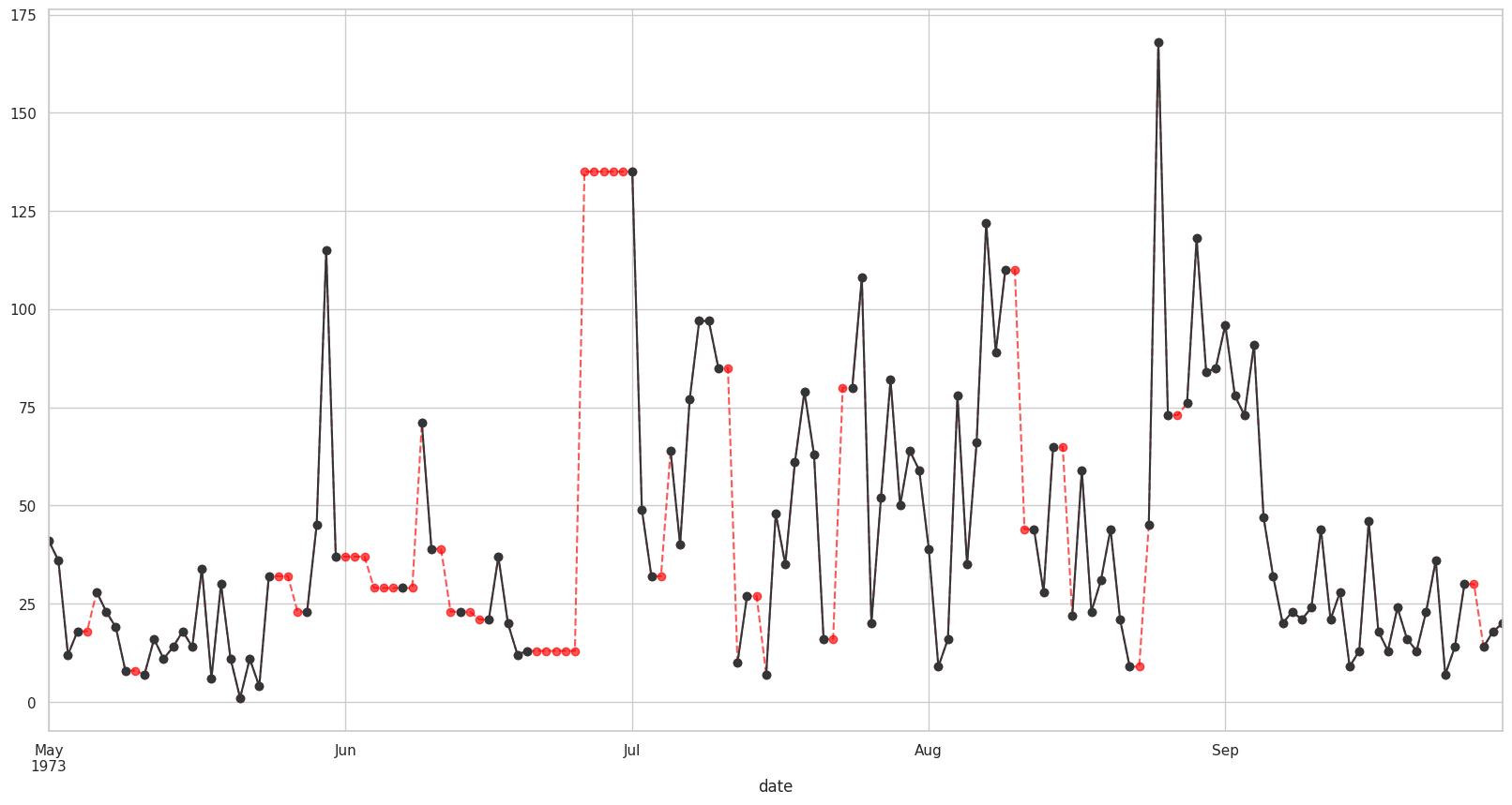
Visualizando con bfill o ffill con valores mas cercanos

plt.figure(figsize=(20,10))

(
    airquality_df
    .select_columns("ozone")
    .pipe(
        lambda df: (
            df.ozone.interpolate(method = "nearest").plot(color= "red", marker="o", alpha=6/9, linestyle="dashed"),
            df.ozone.plot(color = "#313638", marker= "o")
        )
    )
)

(<AxesSubplot: xlabel='date'>, <AxesSubplot: xlabel='date'>)

Visualizando valores interpolados

plt.figure(figsize=(20,10))

(
    airquality_df
    .select_columns("ozone")
    .pipe(
        lambda df: (
            df.ozone.interpolate(method = "linear").plot(color= "red", marker="o", alpha=6/9, linestyle="dashed"),
            df.ozone.plot(color = "#313638", marker= "o")
        )
    )
)

(<AxesSubplot: xlabel='date'>, <AxesSubplot: xlabel='date'>)

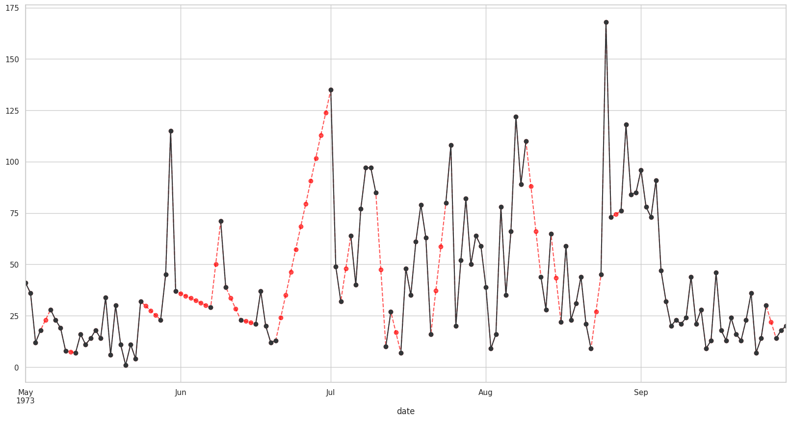
Ahora para asignar esos valores a la columna:

airquality_df["ozone"] = airquality_df.ozone.interpolate(method="linear")

airquality_df

	ozone	solar_r	wind	temp	month	day	year
date
1973-05-01	41.0	190.0	7.4	67	5	1	1973
1973-05-02	36.0	118.0	8.0	72	5	2	1973
1973-05-03	12.0	149.0	12.6	74	5	3	1973
1973-05-04	18.0	313.0	11.5	62	5	4	1973
1973-05-05	23.0	NaN	14.3	56	5	5	1973
...	...	...	...	...	...	...	...
1973-09-26	30.0	193.0	6.9	70	9	26	1973
1973-09-27	22.0	145.0	13.2	77	9	27	1973
1973-09-28	14.0	191.0	14.3	75	9	28	1973
1973-09-29	18.0	131.0	8.0	76	9	29	1973
1973-09-30	20.0	223.0	11.5	68	9	30	1973

153 rows × 7 columns

Imputación por algoritmo de vecinos más cercanos (KNN)

K nearest neighbors (KNN) es el algritmo mas utilizado de imputacion

Resumen de métodos de distancia:

• Euclidiana: Útil para variables numéricas

• Manhattan: Útil paa variables tipo factor

• Hamming: Útil para variables categóricas

• Gower: Útil para conjuntos de datos con variables mixtas

nhanes_transformed_df

	general_health_condition	gender	height	weight	total_cholesterol	pulse	diabetes	age
SEQN
93705.0	2.0	0.0	63.0	165.0	157.0	52.0	0.0	66.0
93706.0	4.0	1.0	68.0	145.0	148.0	82.0	0.0	18.0
93707.0	2.0	1.0	NaN	NaN	189.0	100.0	0.0	13.0
93709.0	NaN	0.0	62.0	200.0	176.0	74.0	0.0	75.0
93711.0	4.0	1.0	69.0	142.0	238.0	62.0	0.0	56.0
...	...	...	...	...	...	...	...	...
102949.0	0.0	1.0	72.0	180.0	201.0	96.0	0.0	33.0
102953.0	1.0	1.0	65.0	218.0	182.0	78.0	0.0	42.0
102954.0	2.0	0.0	66.0	150.0	172.0	78.0	0.0	41.0
102955.0	4.0	0.0	NaN	NaN	150.0	74.0	0.0	14.0
102956.0	2.0	1.0	69.0	250.0	163.0	76.0	0.0	38.0

7157 rows × 8 columns

KNN algorithm

knn_imputer = sklearn.impute.KNNImputer()

#copia del df original
nhanes_df_knn = nhanes_transformed_df.copy(deep=True)

nhanes_df_knn.iloc[:, :] = knn_imputer.fit_transform(nhanes_transformed_df).round()
nhanes_df_knn

	general_health_condition	gender	height	weight	total_cholesterol	pulse	diabetes	age
SEQN
93705.0	2.0	0.0	63.0	165.0	157.0	52.0	0.0	66.0
93706.0	4.0	1.0	68.0	145.0	148.0	82.0	0.0	18.0
93707.0	2.0	1.0	69.0	130.0	189.0	100.0	0.0	13.0
93709.0	2.0	0.0	62.0	200.0	176.0	74.0	0.0	75.0
93711.0	4.0	1.0	69.0	142.0	238.0	62.0	0.0	56.0
...	...	...	...	...	...	...	...	...
102949.0	0.0	1.0	72.0	180.0	201.0	96.0	0.0	33.0
102953.0	1.0	1.0	65.0	218.0	182.0	78.0	0.0	42.0
102954.0	2.0	0.0	66.0	150.0	172.0	78.0	0.0	41.0
102955.0	4.0	0.0	71.0	159.0	150.0	74.0	0.0	14.0
102956.0	2.0	1.0	69.0	250.0	163.0	76.0	0.0	38.0

7157 rows × 8 columns

(
    pd.concat(
        [
            nhanes_df_knn,
            nhanes_df.missing.create_shadow_matrix(True, False, suffix="_imp", only_missing=True)
        ],
        axis=1
    )
)

	general_health_condition	gender	height	weight	total_cholesterol	pulse	diabetes	age	height_imp	weight_imp	general_health_condition_imp	total_cholesterol_imp	pulse_imp
SEQN
93705.0	2.0	0.0	63.0	165.0	157.0	52.0	0.0	66.0	False	False	False	False	False
93706.0	4.0	1.0	68.0	145.0	148.0	82.0	0.0	18.0	False	False	False	False	False
93707.0	2.0	1.0	69.0	130.0	189.0	100.0	0.0	13.0	True	True	False	False	False
93709.0	2.0	0.0	62.0	200.0	176.0	74.0	0.0	75.0	False	False	True	False	False
93711.0	4.0	1.0	69.0	142.0	238.0	62.0	0.0	56.0	False	False	False	False	False
...	...	...	...	...	...	...	...	...	...	...	...	...	...
102949.0	0.0	1.0	72.0	180.0	201.0	96.0	0.0	33.0	False	False	False	False	False
102953.0	1.0	1.0	65.0	218.0	182.0	78.0	0.0	42.0	False	False	False	False	False
102954.0	2.0	0.0	66.0	150.0	172.0	78.0	0.0	41.0	False	False	False	False	False
102955.0	4.0	0.0	71.0	159.0	150.0	74.0	0.0	14.0	True	True	False	False	False
102956.0	2.0	1.0	69.0	250.0	163.0	76.0	0.0	38.0	False	False	False	False	False

7157 rows × 13 columns

(
    pd.concat(
        [
            nhanes_df_knn,
            nhanes_df.missing.create_shadow_matrix(True, False, suffix="_imp", only_missing=True)
        ],
        axis=1
    )
    .missing.scatter_imputation_plot(
        x = "height",
        y = "weight"
    )
)

<AxesSubplot: xlabel='height', ylabel='weight'>

Ordenamiento por cantidad de variables faltantes

knn_imputer = sklearn.impute.KNNImputer()

#copia del df original
nhanes_df_knn = nhanes_transformed_df.missing.sort_variables_by_missingness(ascending=True).copy(deep=True)

nhanes_df_knn.iloc[:, :] = knn_imputer.fit_transform(nhanes_transformed_df.missing.sort_variables_by_missingness(ascending=True)).round()
nhanes_df_knn

	gender	diabetes	age	pulse	total_cholesterol	general_health_condition	weight	height
SEQN
93705.0	0.0	0.0	66.0	52.0	157.0	2.0	165.0	63.0
93706.0	1.0	0.0	18.0	82.0	148.0	4.0	145.0	68.0
93707.0	1.0	0.0	13.0	100.0	189.0	2.0	130.0	69.0
93709.0	0.0	0.0	75.0	74.0	176.0	2.0	200.0	62.0
93711.0	1.0	0.0	56.0	62.0	238.0	4.0	142.0	69.0
...	...	...	...	...	...	...	...	...
102949.0	1.0	0.0	33.0	96.0	201.0	0.0	180.0	72.0
102953.0	1.0	0.0	42.0	78.0	182.0	1.0	218.0	65.0
102954.0	0.0	0.0	41.0	78.0	172.0	2.0	150.0	66.0
102955.0	0.0	0.0	14.0	74.0	150.0	4.0	159.0	71.0
102956.0	1.0	0.0	38.0	76.0	163.0	2.0	250.0	69.0

7157 rows × 8 columns

(
    pd.concat(
        [
            nhanes_df_knn,
            nhanes_df.missing.create_shadow_matrix(True, False, suffix="_imp", only_missing=True)
        ],
        axis=1
    )
    .missing.scatter_imputation_plot(
        x = "height",
        y = "weight"
    )
)

<AxesSubplot: xlabel='height', ylabel='weight'>

Imputación basada en modelos

nhanes_model_df = (
    nhanes_df
    .select_columns("height", "weight", "gender", "age")
    .sort_values("weight")
    .transform_column(
        "weight",
        lambda x: x.ffill(),
        elementwise = False
    )
    .missing.bind_shadow_matrix(
        True,
        False,
        suffix="_imp",
        only_missing = False
    )
)

nhanes_model_df

	height	weight	gender	age	height_imp	weight_imp	gender_imp	age_imp
SEQN
99970.0	62.0	72.0	Male	16.0	False	False	False	False
97877.0	50.0	80.0	Female	29.0	False	False	False	False
96451.0	59.0	82.0	Female	80.0	False	False	False	False
97730.0	62.0	82.0	Female	19.0	False	False	False	False
99828.0	62.0	85.0	Female	16.0	False	False	False	False
...	...	...	...	...	...	...	...	...
102915.0	NaN	484.0	Female	14.0	True	False	False	False
102926.0	NaN	484.0	Female	15.0	True	False	False	False
102941.0	NaN	484.0	Female	14.0	True	False	False	False
102945.0	NaN	484.0	Male	15.0	True	False	False	False
102955.0	NaN	484.0	Female	14.0	True	False	False	False

7157 rows × 8 columns

height_ols = (
    nhanes_model_df
    .pipe(
        lambda df: smf.ols("height ~ weight + age", data=df)
    )
    .fit()
)

ols_imputed_values = (
    nhanes_model_df
    .pipe(
        lambda df: df[df.height.isna()]
    )
    .pipe(
        lambda df: height_ols.predict(df).round()
    )
)

ols_imputed_values

SEQN
100246.0    64.0
101209.0    64.0
102766.0    64.0
102509.0    64.0
96900.0     65.0
            ... 
102915.0    75.0
102926.0    75.0
102941.0    75.0
102945.0    75.0
102955.0    75.0
Length: 1669, dtype: float64

nhanes_model_df.loc[nhanes_model_df.height.isna(), ["height"]] = ols_imputed_values
nhanes_model_df

	height	weight	gender	age	height_imp	weight_imp	gender_imp	age_imp
SEQN
99970.0	62.0	72.0	Male	16.0	False	False	False	False
97877.0	50.0	80.0	Female	29.0	False	False	False	False
96451.0	59.0	82.0	Female	80.0	False	False	False	False
97730.0	62.0	82.0	Female	19.0	False	False	False	False
99828.0	62.0	85.0	Female	16.0	False	False	False	False
...	...	...	...	...	...	...	...	...
102915.0	75.0	484.0	Female	14.0	True	False	False	False
102926.0	75.0	484.0	Female	15.0	True	False	False	False
102941.0	75.0	484.0	Female	14.0	True	False	False	False
102945.0	75.0	484.0	Male	15.0	True	False	False	False
102955.0	75.0	484.0	Female	14.0	True	False	False	False

7157 rows × 8 columns

(
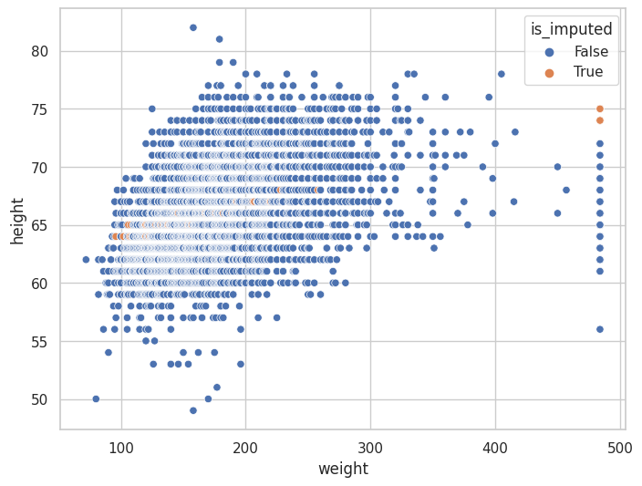
    nhanes_model_df
    .missing.scatter_imputation_plot(
        x = "weight",
        y = "height"
    )
)

<AxesSubplot: xlabel='weight', ylabel='height'>

Imputaciones Múltiples por Ecuaciones Encadenadas (MICE)

mice_imputer = sklearn.impute.IterativeImputer(
    estimator=BayesianRidge(),
    initial_strategy="mean",
    imputation_order="ascending"
)

nhanes_mice_df = nhanes_transformed_df.copy(deep=True)

nhanes_mice_df.iloc[:, :] = mice_imputer.fit_transform(nhanes_transformed_df).round()

nhanes_mice_df = pd.concat(
    [
        nhanes_mice_df,
        nhanes_df.missing.create_shadow_matrix(True, False, suffix="_imp")
    ],    
    axis=1
)

nhanes_mice_df

	general_health_condition	gender	height	weight	total_cholesterol	pulse	diabetes	age	height_imp	weight_imp	general_health_condition_imp	total_cholesterol_imp	pulse_imp	diabetes_imp	age_imp	gender_imp
SEQN
93705.0	2.0	0.0	63.0	165.0	157.0	52.0	0.0	66.0	False	False	False	False	False	False	False	False
93706.0	4.0	1.0	68.0	145.0	148.0	82.0	0.0	18.0	False	False	False	False	False	False	False	False
93707.0	2.0	1.0	70.0	200.0	189.0	100.0	0.0	13.0	True	True	False	False	False	False	False	False
93709.0	2.0	0.0	62.0	200.0	176.0	74.0	0.0	75.0	False	False	True	False	False	False	False	False
93711.0	4.0	1.0	69.0	142.0	238.0	62.0	0.0	56.0	False	False	False	False	False	False	False	False
...	...	...	...	...	...	...	...	...	...	...	...	...	...	...	...	...
102949.0	0.0	1.0	72.0	180.0	201.0	96.0	0.0	33.0	False	False	False	False	False	False	False	False
102953.0	1.0	1.0	65.0	218.0	182.0	78.0	0.0	42.0	False	False	False	False	False	False	False	False
102954.0	2.0	0.0	66.0	150.0	172.0	78.0	0.0	41.0	False	False	False	False	False	False	False	False
102955.0	4.0	0.0	64.0	159.0	150.0	74.0	0.0	14.0	True	True	False	False	False	False	False	False
102956.0	2.0	1.0	69.0	250.0	163.0	76.0	0.0	38.0	False	False	False	False	False	False	False	False

7157 rows × 16 columns

nhanes_mice_df.missing.scatter_imputation_plot(
    x = "height",
    y = "weight"
)

<AxesSubplot: xlabel='height', ylabel='weight'>

Transformación inversa de los datos

Deshacer la transformacion en dummy

nhanes_imputed_df = nhanes_mice_df.copy(deep=True)

nhanes_imputed_df[categorical_columns] = (
    categorical_transformer
    .named_transformers_
    .ordinalencoder
    .inverse_transform(
        X = nhanes_mice_df[categorical_columns]
    )
)

nhanes_imputed_df

	general_health_condition	gender	height	weight	total_cholesterol	pulse	diabetes	age	height_imp	weight_imp	general_health_condition_imp	total_cholesterol_imp	pulse_imp	diabetes_imp	age_imp	gender_imp
SEQN
93705.0	Good	Female	63.0	165.0	157.0	52.0	0.0	66.0	False	False	False	False	False	False	False	False
93706.0	Very good	Male	68.0	145.0	148.0	82.0	0.0	18.0	False	False	False	False	False	False	False	False
93707.0	Good	Male	70.0	200.0	189.0	100.0	0.0	13.0	True	True	False	False	False	False	False	False
93709.0	Good	Female	62.0	200.0	176.0	74.0	0.0	75.0	False	False	True	False	False	False	False	False
93711.0	Very good	Male	69.0	142.0	238.0	62.0	0.0	56.0	False	False	False	False	False	False	False	False
...	...	...	...	...	...	...	...	...	...	...	...	...	...	...	...	...
102949.0	Excellent	Male	72.0	180.0	201.0	96.0	0.0	33.0	False	False	False	False	False	False	False	False
102953.0	Fair or	Male	65.0	218.0	182.0	78.0	0.0	42.0	False	False	False	False	False	False	False	False
102954.0	Good	Female	66.0	150.0	172.0	78.0	0.0	41.0	False	False	False	False	False	False	False	False
102955.0	Very good	Female	64.0	159.0	150.0	74.0	0.0	14.0	True	True	False	False	False	False	False	False
102956.0	Good	Male	69.0	250.0	163.0	76.0	0.0	38.0	False	False	False	False	False	False	False	False

7157 rows × 16 columns

Comparativa de valores antes de imputacion con valores despues de imputacion

nhanes_df.general_health_condition.value_counts()

Good         2383
Very good    1503
Fair or      1130
Excellent     612
Poor?         169
Name: general_health_condition, dtype: int64

nhanes_imputed_df.general_health_condition.value_counts()

Good         3743
Very good    1503
Fair or      1130
Excellent     612
Poor?         169
Name: general_health_condition, dtype: int64

Me quedan entonces valores faltantes?

nhanes_imputed_df.missing.number_missing()

0

Created in Deepnote