Inferential Statistics & Sampling

Sampling

Samples are extracted from the population and must meet two requirements:

• Must be statistically significant (big enough to take conclusion)

• not biased

There are 3 types of sampling:

• simple random sampling

• systematic sampling

• stratified sampling

pip install -r requirements.txt

^C

Collecting pingouin==0.5.3 (from -r requirements.txt (line 1))
  Using cached pingouin-0.5.3-py3-none-any.whl (198 kB)
Requirement already satisfied: numpy>=1.19 in c:\users\admin\miniconda3\lib\site-packages (from pingouin==0.5.3->-r requirements.txt (line 1)) (1.25.2)
Requirement already satisfied: scipy>=1.7 in c:\users\admin\miniconda3\lib\site-packages (from pingouin==0.5.3->-r requirements.txt (line 1)) (1.11.2)
Requirement already satisfied: pandas>=1.0 in c:\users\admin\miniconda3\lib\site-packages (from pingouin==0.5.3->-r requirements.txt (line 1)) (2.1.0)
Collecting matplotlib>=3.0.2 (from pingouin==0.5.3->-r requirements.txt (line 1))
  Using cached matplotlib-3.7.2-cp311-cp311-win_amd64.whl (7.5 MB)
Collecting seaborn>=0.11 (from pingouin==0.5.3->-r requirements.txt (line 1))
  Using cached seaborn-0.12.2-py3-none-any.whl (293 kB)
Collecting statsmodels>=0.13 (from pingouin==0.5.3->-r requirements.txt (line 1))
  Using cached statsmodels-0.14.0-cp311-cp311-win_amd64.whl (9.2 MB)
Requirement already satisfied: scikit-learn in c:\users\admin\miniconda3\lib\site-packages (from pingouin==0.5.3->-r requirements.txt (line 1)) (1.3.0)
Collecting pandas-flavor>=0.2.0 (from pingouin==0.5.3->-r requirements.txt (line 1))
  Using cached pandas_flavor-0.6.0-py3-none-any.whl (7.2 kB)
Collecting outdated (from pingouin==0.5.3->-r requirements.txt (line 1))
  Using cached outdated-0.2.2-py2.py3-none-any.whl (7.5 kB)
Requirement already satisfied: tabulate in c:\users\admin\miniconda3\lib\site-packages (from pingouin==0.5.3->-r requirements.txt (line 1)) (0.9.0)
Requirement already satisfied: contourpy>=1.0.1 in c:\users\admin\miniconda3\lib\site-packages (from matplotlib>=3.0.2->pingouin==0.5.3->-r requirements.txt (line 1)) (1.1.0)
Requirement already satisfied: cycler>=0.10 in c:\users\admin\miniconda3\lib\site-packages (from matplotlib>=3.0.2->pingouin==0.5.3->-r requirements.txt (line 1)) (0.11.0)
Requirement already satisfied: fonttools>=4.22.0 in c:\users\admin\miniconda3\lib\site-packages (from matplotlib>=3.0.2->pingouin==0.5.3->-r requirements.txt (line 1)) (4.42.1)
Requirement already satisfied: kiwisolver>=1.0.1 in c:\users\admin\miniconda3\lib\site-packages (from matplotlib>=3.0.2->pingouin==0.5.3->-r requirements.txt (line 1)) (1.4.5)
Requirement already satisfied: packaging>=20.0 in c:\users\admin\miniconda3\lib\site-packages (from matplotlib>=3.0.2->pingouin==0.5.3->-r requirements.txt (line 1)) (23.0)
Requirement already satisfied: pillow>=6.2.0 in c:\users\admin\miniconda3\lib\site-packages (from matplotlib>=3.0.2->pingouin==0.5.3->-r requirements.txt (line 1)) (10.0.0)
Requirement already satisfied: pyparsing<3.1,>=2.3.1 in c:\users\admin\miniconda3\lib\site-packages (from matplotlib>=3.0.2->pingouin==0.5.3->-r requirements.txt (line 1)) (3.0.9)
Requirement already satisfied: python-dateutil>=2.7 in c:\users\admin\miniconda3\lib\site-packages (from matplotlib>=3.0.2->pingouin==0.5.3->-r requirements.txt (line 1)) (2.8.2)
Requirement already satisfied: pytz>=2020.1 in c:\users\admin\miniconda3\lib\site-packages (from pandas>=1.0->pingouin==0.5.3->-r requirements.txt (line 1)) (2023.3.post1)
Requirement already satisfied: tzdata>=2022.1 in c:\users\admin\miniconda3\lib\site-packages (from pandas>=1.0->pingouin==0.5.3->-r requirements.txt (line 1)) (2023.3)
Collecting xarray (from pandas-flavor>=0.2.0->pingouin==0.5.3->-r requirements.txt (line 1))
  Using cached xarray-2023.8.0-py3-none-any.whl (1.0 MB)
Requirement already satisfied: patsy>=0.5.2 in c:\users\admin\miniconda3\lib\site-packages (from statsmodels>=0.13->pingouin==0.5.3->-r requirements.txt (line 1)) (0.5.3)
Requirement already satisfied: setuptools>=44 in c:\users\admin\miniconda3\lib\site-packages (from outdated->pingouin==0.5.3->-r requirements.txt (line 1)) (67.8.0)
Requirement already satisfied: littleutils in c:\users\admin\miniconda3\lib\site-packages (from outdated->pingouin==0.5.3->-r requirements.txt (line 1)) (0.2.2)
Requirement already satisfied: requests in c:\users\admin\miniconda3\lib\site-packages (from outdated->pingouin==0.5.3->-r requirements.txt (line 1)) (2.29.0)
Requirement already satisfied: joblib>=1.1.1 in c:\users\admin\miniconda3\lib\site-packages (from scikit-learn->pingouin==0.5.3->-r requirements.txt (line 1)) (1.3.2)
Requirement already satisfied: threadpoolctl>=2.0.0 in c:\users\admin\miniconda3\lib\site-packages (from scikit-learn->pingouin==0.5.3->-r requirements.txt (line 1)) (3.2.0)
Requirement already satisfied: six in c:\users\admin\miniconda3\lib\site-packages (from patsy>=0.5.2->statsmodels>=0.13->pingouin==0.5.3->-r requirements.txt (line 1)) (1.16.0)
Requirement already satisfied: charset-normalizer<4,>=2 in c:\users\admin\miniconda3\lib\site-packages (from requests->outdated->pingouin==0.5.3->-r requirements.txt (line 1)) (2.0.4)
Requirement already satisfied: idna<4,>=2.5 in c:\users\admin\miniconda3\lib\site-packages (from requests->outdated->pingouin==0.5.3->-r requirements.txt (line 1)) (3.4)
Requirement already satisfied: urllib3<1.27,>=1.21.1 in c:\users\admin\miniconda3\lib\site-packages (from requests->outdated->pingouin==0.5.3->-r requirements.txt (line 1)) (1.26.16)
Requirement already satisfied: certifi>=2017.4.17 in c:\users\admin\miniconda3\lib\site-packages (from requests->outdated->pingouin==0.5.3->-r requirements.txt (line 1)) (2023.5.7)
Installing collected packages: outdated, matplotlib, xarray, statsmodels, seaborn, pandas-flavor, pingouin

Note: you may need to restart the kernel to use updated packages.

import numpy as np
import pandas as pd
import matplotlib.pyplot as plt
import seaborn as sns
import random
import io
import math
from scipy.stats import norm
from scipy.stats import t
import scipy.stats as stats
import pingouin

Database to work

Database of the mexican government, contains information about hotels, museums and marketplaces at “El centro historico de la Ciudad de Mexico”

econdata = pd.read_csv("econdata.csv")

econdata.head()

	id	geo_point_2d	geo_shape	clave_cat	delegacion	perimetro	tipo	nom_id
0	0	19.424781053,-99.1327537959	{"type": "Polygon", "coordinates": [[[-99.1332...	307_130_11	Cuauhtémoc	B	Mercado	Pino Suárez
1	1	19.4346139576,-99.1413808393	{"type": "MultiPoint", "coordinates": [[-99.14...	002_008_01	Cuautémoc	A	Museo	Museo Nacional de Arquitectura Palacio de Bell...
2	2	19.4340695945,-99.1306348409	{"type": "MultiPoint", "coordinates": [[-99.13...	006_002_12	Cuautémoc	A	Museo	Santa Teresa
3	3	19.42489472,-99.12073393	{"type": "MultiPoint", "coordinates": [[-99.12...	323_102_06	Venustiano Carranza	B	Hotel	Balbuena
4	4	19.42358238,-99.12451093	{"type": "MultiPoint", "coordinates": [[-99.12...	323_115_12	Venustiano Carranza	B	Hotel	real

Types of sampling

Simple random sampling

This technique consists of just extracting completely random samples

rand1 = econdata.sample(n=8)
rand1

	id	geo_point_2d	geo_shape	clave_cat	delegacion	perimetro	tipo	nom_id
30	30	19.427530818,-99.1479200065	{"type": "MultiPoint", "coordinates": [[-99.14...	002_068_13	Cuautémoc	B	Hotel	Villa Pal
103	103	19.4370810464,-99.1361494106	{"type": "MultiPoint", "coordinates": [[-99.13...	004_091_27	Cuautémoc	A	Hotel	Cuba
145	145	19.4340221684,-99.1358187396	{"type": "MultiPoint", "coordinates": [[-99.13...	001_012_11	Cuautémoc	A	Hotel	Rioja
65	65	19.425466805,-99.1380880561	{"type": "MultiPoint", "coordinates": [[-99.13...	001_073_20	Cuautémoc	B	Hotel	Mar
125	125	19.4342350395,-99.1354548065	{"type": "MultiPoint", "coordinates": [[-99.13...	001_007_06	Cuautémoc	A	Hotel	Zamora
25	25	19.42477346,-99.12881894	{"type": "MultiPoint", "coordinates": [[-99.12...	307_123_30	Cuautémoc	B	Hotel	Madrid
111	111	19.4430614318,-99.1353793874	{"type": "MultiPoint", "coordinates": [[-99.13...	004_107_02	Cuautémoc	B	Hotel	Embajadores
59	59	19.4275850427,-99.1397624613	{"type": "MultiPoint", "coordinates": [[-99.13...	001_061_03	Cuautémoc	A	Hotel	Señorial

You can do it by specifying a seed

Example:

set a seed: 18900217

rand2 = econdata.sample(n=8, random_state=18900217)
rand2

	id	geo_point_2d	geo_shape	clave_cat	delegacion	perimetro	tipo	nom_id
69	69	19.43558625,-99.12965746	{"type": "MultiPoint", "coordinates": [[-99.12...	005_129_08	Cuautémoc	A	Hotel	Templo Mayor
180	180	19.4357633849,-99.1330511805	{"type": "MultiPoint", "coordinates": [[-99.13...	004_094_32	Cuautémoc	A	Hotel	Catedral, S.A. DE C.V.
25	25	19.42477346,-99.12881894	{"type": "MultiPoint", "coordinates": [[-99.12...	307_123_30	Cuautémoc	B	Hotel	Madrid
83	83	19.4342251093,-99.1449434443	{"type": "MultiPoint", "coordinates": [[-99.14...	002_018_03	Cuautémoc	B	Hotel	San Francisco
27	27	19.4348360773,-99.1463945583	{"type": "MultiPoint", "coordinates": [[-99.14...	002_016_01	Cuautémoc	B	Hotel	Hilton Centro Histórico
181	181	19.4451852396,-99.1478597989	{"type": "MultiPoint", "coordinates": [[-99.14...	012_103_01	Cuautémoc	B	Hotel	Yale
117	117	19.4253041176,-99.1405962735	{"type": "MultiPoint", "coordinates": [[-99.14...	001_078_03	Cuautémoc	B	Hotel	Mazatlán
182	182	19.42407591,-99.1424737531	{"type": "MultiPoint", "coordinates": [[-99.14...	001_094_26	Cuautémoc	B	Hotel	Macao

# Extract a random 25% of your population

prop_25 = econdata.sample(frac = .25)
prop_25

	id	geo_point_2d	geo_shape	clave_cat	delegacion	perimetro	tipo	nom_id
61	61	19.4343847692,-99.125125489	{"type": "Polygon", "coordinates": [[[-99.1257...	005_140_01	Cuauhtémoc	B	Mercado	Mixcalco
138	138	19.4330991176,-99.1423784309	{"type": "MultiPoint", "coordinates": [[-99.14...	002_024_08	Cuautémoc	B	Hotel	Marlowe
33	33	19.4341938751,-99.1352210651	{"type": "MultiPoint", "coordinates": [[-99.13...	001_007_04	Cuautémoc	A	Hotel	Washingtonw
178	178	19.4457531395,-99.1485982115	{"type": "MultiPoint", "coordinates": [[-99.14...	012_069_11	Cuautémoc	B	Hotel	Norte
3	3	19.42489472,-99.12073393	{"type": "MultiPoint", "coordinates": [[-99.12...	323_102_06	Venustiano Carranza	B	Hotel	Balbuena
161	161	19.4356652812,-99.1386591361	{"type": "MultiPoint", "coordinates": [[-99.13...	001_003_12	Cuautémoc	A	Museo	La Tortura
190	190	19.43311885,-99.14512643	{"type": "MultiPoint", "coordinates": [[-99.14...	002_019_02	Cuautémoc	B	Hotel	Metropol
124	124	19.4297560476,-99.1253498219	{"type": "MultiPoint", "coordinates": [[-99.12...	006_052_01	Cuautémoc	A	Hotel	Universo
63	63	19.4339116282,-99.1468371035	{"type": "MultiPoint", "coordinates": [[-99.14...	002_015_07	Cuautémoc	B	Hotel	Calvin
229	229	19.4346765421,-99.1318394918	{"type": "MultiPoint", "coordinates": [[-99.13...	005_145_14	Cuautémoc	A	Museo	Templo Mayor
70	70	19.43712772,-99.1378899	{"type": "MultiPoint", "coordinates": [[-99.13...	004_090_02	Cuautémoc	A	Hotel	Congreso
195	195	19.4414840739,-99.1394736635	{"type": "MultiPoint", "coordinates": [[-99.13...	004_050_13	Cuautémoc	B	Hotel	Emperador
12	12	19.43990186,-99.14813347	{"type": "MultiPoint", "coordinates": [[-99.14...	003_079_16	Cuautémoc	B	Hotel	La Paz
191	191	19.43985567,-99.14782916	{"type": "MultiPoint", "coordinates": [[-99.14...	003_079_12	Cuautémoc	B	Hotel	Ferrol
11	11	19.4219963186,-99.1437414652	{"type": "MultiPoint", "coordinates": [[-99.14...	002_103_18	Cuautémoc	B	Hotel	Faro
113	113	19.43374405,-99.13550135	{"type": "MultiPoint", "coordinates": [[-99.13...	001_012_13	Cuautémoc	A	Hotel	San Antonio
149	149	19.43031663,-99.12465191	{"type": "MultiPoint", "coordinates": [[-99.12...	323_035_01	Venustiano Carranza	B	Hotel	Liverpool
26	26	19.4262321913,-99.1238893146	{"type": "Polygon", "coordinates": [[[-99.1241...	323_064_01	Venustiano Carranza	B	Mercado	La Merced Nave Mayor
78	78	19.4430578017,-99.13614342	{"type": "Polygon", "coordinates": [[[-99.1368...	004_107_01	Cuauhtémoc	B	Mercado	La Lagunilla
37	37	19.4271233834,-99.125111772	{"type": "Polygon", "coordinates": [[[-99.1251...	323_065_01	Venustiano Carranza	B	Mercado	Dulceria
42	42	19.4368553413,-99.1196435872	{"type": "MultiPoint", "coordinates": [[-99.11...	018_337_01	Venustiano Carranza	B	Hotel	HOTEL RRO MI1O
146	146	19.4373584031,-99.1383047535	{"type": "MultiPoint", "coordinates": [[-99.13...	004_090_14	Cuautémoc	A	Hotel	Congreso Garage
130	130	19.4351458312,-99.1282270238	{"type": "MultiPoint", "coordinates": [[-99.12...	005_114_34	Cuautémoc	A	Museo	Sinagoga Histórica de Justo Sierra
81	81	19.42262452,-99.15107339	{"type": "MultiPoint", "coordinates": [[-99.15...	002_096_02	Cuautémoc	B	Hotel	Imperio
82	82	19.4220369889,-99.120775543	{"type": "MultiPoint", "coordinates": [[-99.12...	423_013_18	Venustiano Carranza	B	Hotel	Cordoba
142	142	19.4263681354,-99.1327278126	{"type": "MultiPoint", "coordinates": [[-99.13...	006_127_14	Cuautémoc	A	Hotel	Ambar
226	226	19.4416748524,-99.1365878489	{"type": "Polygon", "coordinates": [[[-99.1370...	004_052_01	Cuauhtémoc	B	Mercado	De Muebles
175	175	19.4291934671,-99.1323328561	{"type": "MultiPoint", "coordinates": [[-99.13...	006_073_11	Cuautémoc	A	Museo	La Ciudad de México
123	123	19.4378770032,-99.1358867181	{"type": "MultiPoint", "coordinates": [[-99.13...	004_086_36	Cuautémoc	A	Hotel	Florida
68	68	19.4273142523,-99.1255788881	{"type": "MultiPoint", "coordinates": [[-99.12...	006_082_02	Cuautémoc	A	Hotel	Anpudia
126	126	19.42774805,-99.12796532	{"type": "MultiPoint", "coordinates": [[-99.12...	006_078_04	Cuautémoc	A	Hotel	San Marcos
136	136	19.4263840955,-99.1429192037	{"type": "MultiPoint", "coordinates": [[-99.14...	002_084_14	Cuautémoc	B	Hotel	Miguel Ángel
153	153	19.4241764183,-99.1254198454	{"type": "MultiPoint", "coordinates": [[-99.12...	323_133_29	Venustiano Carranza	B	Hotel	Navio
39	39	19.4369818158,-99.1426877718	{"type": "MultiPoint", "coordinates": [[-99.14...	003_095_04	Cuautémoc	A	Museo	Museo Nacional de La Estampa
194	194	19.4288786806,-99.1456731565	{"type": "MultiPoint", "coordinates": [[-99.14...	002_060_04	Cuautémoc	B	Hotel	San Diego, S.A. DE C.V.
107	107	19.4248237343,-99.1311696681	{"type": "Polygon", "coordinates": [[[-99.1313...	307_128_04	Cuauhtémoc	B	Mercado	San Lucas
135	135	19.4300009578,-99.1430773295	{"type": "Polygon", "coordinates": [[[-99.1431...	002_045_01	Cuauhtémoc	B	Mercado	Centro Artesanal "San Juan"
50	50	19.427412415,-99.1425547699	{"type": "Polygon", "coordinates": [[[-99.1427...	002_064_05	Cuauhtémoc	B	Mercado	San Juan No.78
99	99	19.4438918423,-99.1402516182	{"type": "MultiPoint", "coordinates": [[-99.14...	003_052_18	Cuautémoc	B	Hotel	Drigales
211	211	19.4325804122,-99.146356862	{"type": "MultiPoint", "coordinates": [[-99.14...	002_032_01	Cuautémoc	B	Hotel	Fleming
159	159	19.4337392469,-99.1311991819	{"type": "MultiPoint", "coordinates": [[-99.13...	006_001_06	Cuautémoc	A	Museo	Arte de la Secretaria de Hacienda y Credito Pu...
207	207	19.4344738803,-99.1305689118	{"type": "MultiPoint", "coordinates": [[-99.13...	006_002_13	Cuautémoc	A	Museo	Autonomía Universitaria
179	179	19.421906236,-99.1246612487	{"type": "Polygon", "coordinates": [[[-99.1250...	423_006_01	Venustiano Carranza	B	Mercado	Mercado Sonora
6	6	19.43553422,-99.12324801	{"type": "MultiPoint", "coordinates": [[-99.12...	318_116_11	Venustiano Carranza	B	Hotel	San Antonio Tomatlan
7	7	19.436244494,-99.1477350326	{"type": "MultiPoint", "coordinates": [[-99.14...	002_004-03	Cuautémoc	B	Hotel	Fontan Reforma
65	65	19.425466805,-99.1380880561	{"type": "MultiPoint", "coordinates": [[-99.13...	001_073_20	Cuautémoc	B	Hotel	Mar
215	215	19.4383767258,-99.1331865203	{"type": "MultiPoint", "coordinates": [[-99.13...	004_082_16	Cuautémoc	A	Hotel	La Fontelina , S.A. DE C.V.
223	223	19.4285106481,-99.1367967407	{"type": "MultiPoint", "coordinates": [[-99.13...	001_055_10	Cuautémoc	A	Hotel	Niza
91	91	19.42981826,-99.14607091	{"type": "MultiPoint", "coordinates": [[-99.14...	002_059_01	Cuautémoc	B	Hotel	Pugibet
19	19	19.4317119617,-99.1269115285	{"type": "MultiPoint", "coordinates": [[-99.12...	006_026_28	Cuautémoc	A	Museo	Alondiga La Merced
221	221	19.4386933829,-99.1481075783	{"type": "MultiPoint", "coordinates": [[-99.14...	003_103_26	Cuautémoc	A	Hotel	San Fernando
137	137	19.4421185698,-99.1482841686	{"type": "MultiPoint", "coordinates": [[-99.14...	012_108_03	Cuautémoc	B	Hotel	Lepanto
32	32	19.4369607249,-99.1354098031	{"type": "MultiPoint", "coordinates": [[-99.13...	004_101_20	Cuautémoc	A	Hotel	Habana, S.A.
121	121	19.4303083246,-99.1405735286	{"type": "MultiPoint", "coordinates": [[-99.14...	001_043_15	Cuautémoc	A	Hotel	El Salvador
210	210	19.43082385,-99.12366058	{"type": "MultiPoint", "coordinates": [[-99.12...	323_029_08	Venustiano Carranza	B	Hotel	Hispano
168	168	19.4349726565,-99.147766133	{"type": "MultiPoint", "coordinates": [[-99.14...	002_014_23	Cuautémoc	B	Hotel	One Alameda
100	100	19.4337759404,-99.1378211234	{"type": "MultiPoint", "coordinates": [[-99.13...	001_014_06	Cuautémoc	A	Hotel	Ritz Ciudada de México
196	196	19.4437017048,-99.1325438818	{"type": "MultiPoint", "coordinates": [[-99.13...	004_043_06	Cuautémoc	B	Hotel	Boston

Systematic sampling

This technique extracts samples based on a condition or rule

example:

Let’s define a function to take samples each \(n\) rows

# let's take samples each 3 rows

def systematic_sampling(econdata, step):
    indexes = np.arange(0, len(econdata), step=step)
    systematic_sample = econdata.iloc[indexes]
    return systematic_sample

systematic_sample = systematic_sampling(econdata,3)
systematic_sample.head(20)

	id	geo_point_2d	geo_shape	clave_cat	delegacion	perimetro	tipo	nom_id
0	0	19.424781053,-99.1327537959	{"type": "Polygon", "coordinates": [[[-99.1332...	307_130_11	Cuauhtémoc	B	Mercado	Pino Suárez
3	3	19.42489472,-99.12073393	{"type": "MultiPoint", "coordinates": [[-99.12...	323_102_06	Venustiano Carranza	B	Hotel	Balbuena
6	6	19.43553422,-99.12324801	{"type": "MultiPoint", "coordinates": [[-99.12...	318_116_11	Venustiano Carranza	B	Hotel	San Antonio Tomatlan
9	9	19.4407152937,-99.1498060057	{"type": "MultiPoint", "coordinates": [[-99.14...	012_146_22	Cuautémoc	B	Hotel	Detroit
12	12	19.43990186,-99.14813347	{"type": "MultiPoint", "coordinates": [[-99.14...	003_079_16	Cuautémoc	B	Hotel	La Paz
15	15	19.42413788,-99.1324515	{"type": "MultiPoint", "coordinates": [[-99.13...	307_153_11	Cuautémoc	B	Hotel	San Lucas
18	18	19.4331161255,-99.1309438719	{"type": "MultiPoint", "coordinates": [[-99.13...	006_021_01	Cuautémoc	A	Museo	Museo Nacional de las Culturas
21	21	19.43614459,-99.13945267	{"type": "MultiPoint", "coordinates": [[-99.13...	004_098_01	Cuautémoc	A	Museo	Telégrafo
24	24	19.4285279152,-99.147008562	{"type": "MultiPoint", "coordinates": [[-99.14...	002_067_19	Cuautémoc	B	Hotel	Fornos
27	27	19.4348360773,-99.1463945583	{"type": "MultiPoint", "coordinates": [[-99.14...	002_016_01	Cuautémoc	B	Hotel	Hilton Centro Histórico
30	30	19.427530818,-99.1479200065	{"type": "MultiPoint", "coordinates": [[-99.14...	002_068_13	Cuautémoc	B	Hotel	Villa Pal
33	33	19.4341938751,-99.1352210651	{"type": "MultiPoint", "coordinates": [[-99.13...	001_007_04	Cuautémoc	A	Hotel	Washingtonw
36	36	19.4425777264,-99.1292760518	{"type": "Polygon", "coordinates": [[[-99.1288...	005_077_01	Cuauhtémoc	B	Mercado	Granaditas
39	39	19.4369818158,-99.1426877718	{"type": "MultiPoint", "coordinates": [[-99.14...	003_095_04	Cuautémoc	A	Museo	Museo Nacional de La Estampa
42	42	19.4368553413,-99.1196435872	{"type": "MultiPoint", "coordinates": [[-99.11...	018_337_01	Venustiano Carranza	B	Hotel	HOTEL RRO MI1O
45	45	19.4438839913,-99.1361724518	{"type": "MultiPoint", "coordinates": [[-99.13...	004_040_11	Cuautémoc	B	Hotel	Guadalajara
48	48	19.4454876095,-99.1454023878	{"type": "Polygon", "coordinates": [[[-99.1457...	003_045_01	Cuauhtémoc	B	Mercado	Martínez de la Torre Anexo
51	51	19.4357182545,-99.1308788314	{"type": "MultiPoint", "coordinates": [[-99.13...	005_129_16	Cuautémoc	A	Museo	Antiguo Colegio de San Idelfonso
54	54	19.4263645964,-99.1399088724	{"type": "MultiPoint", "coordinates": [[-99.13...	001_076_12	Cuautémoc	B	Hotel	Cadillac, S.A. DE C.V.
57	57	19.4303913751,-99.1465372648	{"type": "MultiPoint", "coordinates": [[-99.14...	002_048_10	Cuautémoc	B	Hotel	Conde

Samples equally distanced

Now, Let’s take 10 samples equally distanced

sample_size = 10
interval = int( len(econdata) / sample_size )

econdata.iloc[::interval]#.reset_index()

	id	geo_point_2d	geo_shape	clave_cat	delegacion	perimetro	tipo	nom_id
0	0	19.424781053,-99.1327537959	{"type": "Polygon", "coordinates": [[[-99.1332...	307_130_11	Cuauhtémoc	B	Mercado	Pino Suárez
23	23	19.4390916028,-99.1493421468	{"type": "MultiPoint", "coordinates": [[-99.14...	012_147_01	Cuautémoc	B	Hotel	La Fuente
46	46	19.426941681,-99.1326869759	{"type": "MultiPoint", "coordinates": [[-99.13...	006_090_12	Cuautémoc	A	Hotel	Castropol
69	69	19.43558625,-99.12965746	{"type": "MultiPoint", "coordinates": [[-99.12...	005_129_08	Cuautémoc	A	Hotel	Templo Mayor
92	92	19.4383554723,-99.1327563513	{"type": "MultiPoint", "coordinates": [[-99.13...	004_082_19	Cuautémoc	A	Hotel	Tuxpan
115	115	19.4336966991,-99.1237253904	{"type": "MultiPoint", "coordinates": [[-99.12...	323_010_09	Venustiano Carranza	B	Hotel	Antas
138	138	19.4330991176,-99.1423784309	{"type": "MultiPoint", "coordinates": [[-99.14...	002_024_08	Cuautémoc	B	Hotel	Marlowe
161	161	19.4356652812,-99.1386591361	{"type": "MultiPoint", "coordinates": [[-99.13...	001_003_12	Cuautémoc	A	Museo	La Tortura
184	184	19.4306993983,-99.1389056387	{"type": "MultiPoint", "coordinates": [[-99.13...	001_043_01	Cuautémoc	A	Hotel	La Casa de la Luna, S.A. DE C.V.
207	207	19.4344738803,-99.1305689118	{"type": "MultiPoint", "coordinates": [[-99.13...	006_002_13	Cuautémoc	A	Museo	Autonomía Universitaria

Stratified sampling

This type of sampling consists in creating homogeneus exclusive groups and from there, create a random sample

Proportional stratified sample

Suppose you have a dataset and you would like to take a sample that has the same proportions as the population

penguins = sns.load_dataset("penguins")

penguins["species"].value_counts(normalize=True)

Adelie       0.441860
Gentoo       0.360465
Chinstrap    0.197674
Name: species, dtype: float64

In that case you have:

1. Group by the column that contains the proportion

2. Sample using the frac= argument, to base in a proportion

prop_sample = penguins.groupby("species").sample(frac=0.1)

prop_sample["species"].value_counts(normalize=True)

Adelie       0.441176
Gentoo       0.352941
Chinstrap    0.205882
Name: species, dtype: float64

Note that the sample still contains the same proportion than the original dataset does. In addition, it contains a random 10% of the original data

Equal count stratified sampling

This process allows to take an equal number of samples based on a variable

equal_sample = penguins.groupby("species").sample(n=15)

equal_sample["species"].value_counts(normalize=True)

Chinstrap    0.333333
Gentoo       0.333333
Adelie       0.333333
Name: species, dtype: float64

Weighted random sampling

this one adjusts the relative probability of a row being sampled

Example:

Let’s take samples so that Adelie has the double of probability

first you must create a column, assign 2 if the specie is Adelie, otherwise assign 1

condition = penguins["species"] == "Adelie"

penguins["weight"] = np.where(condition, 2, 1)

Now take the sample with the argument weight

penguins_weight = penguins.sample(frac=0.1, weights="weight")

penguins_weight["species"].value_counts(normalize=True)

Adelie       0.676471
Gentoo       0.205882
Chinstrap    0.117647
Name: species, dtype: float64

Proportional stratified sample (given a proportion)

In this case, we are not neccesarily sampling based on a dataset proportion. Now we are going to provide the proportion to our funtion.

# 1st step: Create your stratification variable

econdata["estratificado"] = econdata["delegacion"] + ", " + econdata["tipo"]
(econdata["estratificado"].value_counts()/len(econdata)).sort_values(ascending=False)

Cuautémoc, Hotel                0.643478
Cuautémoc, Museo                0.156522
Venustiano Carranza, Hotel      0.078261
Cuauhtémoc, Mercado             0.073913
Venustiano Carranza, Mercado    0.047826
Name: estratificado, dtype: float64

The output above shows the proportion of the variables in the dataset.

Suppose now you want to extract a sample with the following proportion:

Cuautémoc,Hotel 0.5 Cuautémoc,Museo 0.2 Venustiano Carranza,Hotel 0.1 Cuauhtémoc,Mercado 0.1 Venustiano Carranza,Mercado 0.1

Let’s create a function that can extract a sample with that given proportion.

def stratified_data(econdata, strat_cols, strat_values, strat_prop, random_state=None):
    df_strat = pd.DataFrame(columns=econdata.columns)

    pos = -1
    for i in range(len(strat_values)):
        pos += 1
        if pos == len(strat_values) - 1:
            ratio_len = len(econdata) - len(df_strat)
        else:
            ratio_len = int(len(econdata) * strat_prop[i])

        df_filtered = econdata[econdata[strat_cols] == strat_values[i]]
        df_temp = df_filtered.sample(replace=True, n=ratio_len, random_state=random_state)

        df_strat = pd.concat([df_strat, df_temp])
    return df_strat

strat_values = list(econdata["estratificado"].unique())
strat_prop = [0.5, 0.2, 0.1, 0.1, 0.1]

# Using the function with the given parameters
df_strat = stratified_data(econdata, "estratificado", strat_values, strat_prop, random_state=42)

df_strat

	id	geo_point_2d	geo_shape	clave_cat	delegacion	perimetro	tipo	nom_id	estratificado
78	78	19.4430578017,-99.13614342	{"type": "Polygon", "coordinates": [[[-99.1368...	004_107_01	Cuauhtémoc	B	Mercado	La Lagunilla	Cuauhtémoc, Mercado
162	162	19.4452741596,-99.1443205075	{"type": "Polygon", "coordinates": [[[-99.1448...	003_044_01	Cuauhtémoc	B	Mercado	Martínez de la Torre	Cuauhtémoc, Mercado
129	129	NaN	NaN	005_125_01	Cuauhtémoc	A	Mercado	Abelardo	Cuauhtémoc, Mercado
79	79	19.4299360348,-99.1445730919	{"type": "Polygon", "coordinates": [[[-99.1450...	002_047_11	Cuauhtémoc	B	Mercado	San Juan	Cuauhtémoc, Mercado
78	78	19.4430578017,-99.13614342	{"type": "Polygon", "coordinates": [[[-99.1368...	004_107_01	Cuauhtémoc	B	Mercado	La Lagunilla	Cuauhtémoc, Mercado
...	...	...	...	...	...	...	...	...	...
128	128	19.4270781084,-99.1210175514	{"type": "Polygon", "coordinates": [[[-99.1214...	323_061_04(123)	Venustiano Carranza	B	Mercado	San Ciprian	Venustiano Carranza, Mercado
37	37	19.4271233834,-99.125111772	{"type": "Polygon", "coordinates": [[[-99.1251...	323_065_01	Venustiano Carranza	B	Mercado	Dulceria	Venustiano Carranza, Mercado
163	163	19.4265454033,-99.1224859032	{"type": "Polygon", "coordinates": [[[-99.1231...	323_063_05	Venustiano Carranza	B	Mercado	NaN	Venustiano Carranza, Mercado
156	156	19.4255480371,-99.1249308096	{"type": "Polygon", "coordinates": [[[-99.1253...	323_138_04 (3)	Venustiano Carranza	B	Mercado	Mariscos	Venustiano Carranza, Mercado
37	37	19.4271233834,-99.125111772	{"type": "Polygon", "coordinates": [[[-99.1251...	323_065_01	Venustiano Carranza	B	Mercado	Dulceria	Venustiano Carranza, Mercado

230 rows × 9 columns

let’s confirm if the proportion is the desired

(
    (df_strat["estratificado"].value_counts()/len(econdata))
    .sort_values(ascending=False)
)

Cuauhtémoc, Mercado             0.5
Cuautémoc, Museo                0.2
Venustiano Carranza, Hotel      0.1
Venustiano Carranza, Mercado    0.1
Cuautémoc, Hotel                0.1
Name: estratificado, dtype: float64

Cluster sampling

Cluster sampling consists in taking some subgroups using random sampling

And then use simple random sampling in those groups

Bonus: Calculate mean per categories

Whenever you want to calculate an average for a variable bases on a category, you can use the pandas function groupby(). The expression is:

DataFrame.Groupby(“categorical_variable”)[“Numerical_variable”].mean()

attrition_pop = pd.read_csv("HR-Employee-Attrition.csv")

This database contains some data from Human Resources.

Let’s calculate the average hourly rate based on the field of study:

attrition_pop.groupby("EducationField")["HourlyRate"].mean()

EducationField
Human Resources     60.888889
Life Sciences       66.831683
Marketing           66.150943
Medical             65.280172
Other               62.365854
Technical Degree    66.621212
Name: HourlyRate, dtype: float64

Relative error

This measure calculates the error of our sample compared to the population

Calculate relative error

let’s compare the error of the average hourly rate of all the employees vs the average hourly rate of a random 50 employees sample

# take a 50 rows sample, set the seed to 2022
sample = attrition_pop.sample(n=50, random_state=202)

# mean of the population
pop_mean = attrition_pop["HourlyRate"].mean()
# mean of the sample
sample_mean = sample["HourlyRate"].mean()

# Relative error
(abs(pop_mean-sample_mean)/pop_mean)*100

1.7435473879826704

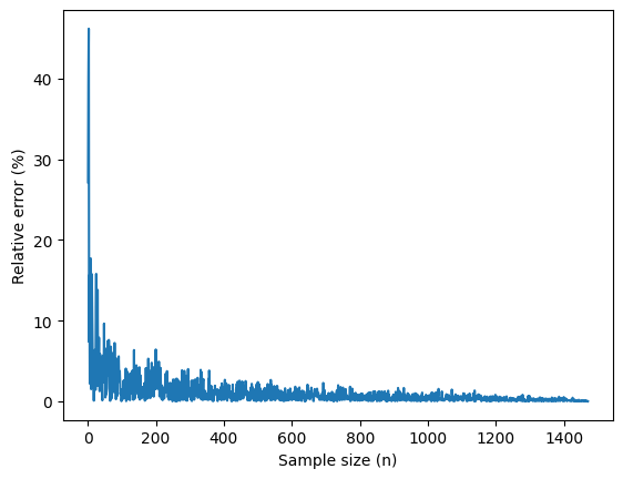
Relative error vs sample size

population_mean = attrition_pop["HourlyRate"].mean()
sample_mean = []
n = []
for i in range(len(attrition_pop["HourlyRate"])):
    sample_mean.append(attrition_pop.sample(n=i+1)["HourlyRate"].mean())
    n.append(i+1)

#Turn sample_mean into a numpy array
sample_mean = np.array(sample_mean)

#Calculate the relative error (%)
rel_error_pct = 100 * abs(population_mean-sample_mean)/population_mean

plt.plot(n, rel_error_pct)
plt.xlabel("Sample size (n)")
plt.ylabel("Relative error (%)")
plt.show()

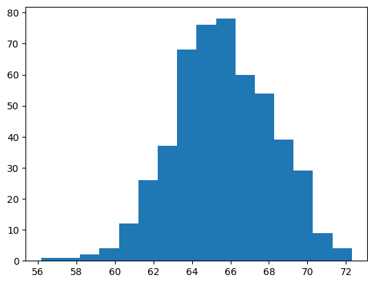
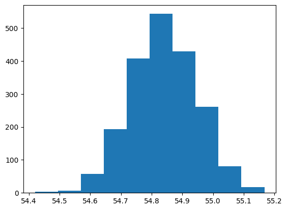
Sampling distribution

Each time you perform a simple random sampling, you will obtain different values for your statistics.

In this example, the sample mean is different each time you repeat the sampling process.

A distribution of replicates of sample means (or other point estimates, is known as a sampling distribution)

mean_hourlyrate = []

for i in range(500):
    mean_hourlyrate.append(
        attrition_pop.sample(n=60)["HourlyRate"].mean()
    )

plt.hist(mean_hourlyrate, bins=16)
plt.show()

Approximating sampling distributions

Sometimes it is computationally imposible to calculate statistics based on a population because it is huge. In those cases, instead of considering all the population, you just take a sample.

In this case, let’s consider the mean value obtained from roll

n_dice = list(range(1, 101))
n_outcomes = []

for n in n_dice:
    n_outcomes.append(6**n)

outcomes = pd.DataFrame(
    {
        "n_dice" : n_dice,
        "n_outcomes" : n_outcomes
    }
)

outcomes.plot(
    x = "n_dice",
    y = "n_outcomes",
    kind = "scatter"
)
plt.show()

/shared-libs/python3.9/py/lib/python3.9/site-packages/pandas/plotting/_matplotlib/core.py:1041: UserWarning: No data for colormapping provided via 'c'. Parameters 'cmap' will be ignored
  scatter = ax.scatter(

Bootstrapping

Concept

When you have a dataset, which clearly doesn’t represent the hold population. You can treat the dataset as a sample and use it to build a theoretical population. this is possible by using a resampling technique whith replacement

Example:

Let’s use the coffee rating dataset. This dataset contains information about professional ratings for different brands of coffees coming from many countries.

Let’s suposse

coffee_ratings = pd.read_csv(
    "https://raw.githubusercontent.com/rfordatascience/tidytuesday/master/data/2020/2020-07-07/coffee_ratings.csv"
)

Let’s use just three columns to make it simple (and store the indexes)

coffee_focus = coffee_ratings[["variety", "country_of_origin", "flavor"]].reset_index()

and now let’s take a sample

coffee_resamp = coffee_focus.sample(frac=1, replace=True)

#frac=1 makes the sample size as big as the dataset

Now see that there are some repeated values, and some others were not even sampled

coffee_resamp["index"].value_counts()

822     5
906     5
809     5
1235    5
1284    4
       ..
537     1
539     1
541     1
542     1
1337    1
Name: index, Length: 850, dtype: int64

How many records didn’t end up in the resample dataset?

len(coffee_ratings) - len(coffee_resamp.drop_duplicates(subset="index"))

489

☝️☝️☝️☝️ this is the amount of samples that didn’t end up in the resample (for this random resample)

Now, what if we extract the mean of this resample, it would be

np.mean(coffee_resamp["flavor"])

7.514794622852876

Actually Bootstrapping

AND NOW LET’S REPEAT THIS PROCESS 1000 TIMES AND SAVE THE MEAN VALUES THAT WE GET FOR EACH RESAMPLE

AND THEN LET’S PLOT THAT TO SEE WHAT HAPPENS

means = []

for i in range(1000):
    means.append(
        np.mean(
            coffee_focus.sample(frac=1, replace=True)["flavor"]
        )
    )

plt.hist(means)
plt.show()

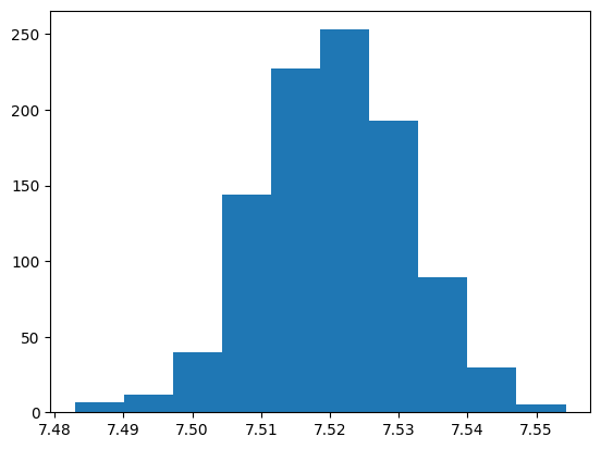
What we have calculated is known as the Bootstrap distribution for the sample mean

1. Make a resample of the same size as the original sample

2. Calculate the statistic of interest for this bootstrap sample

3. PUT THAT INTO A FOR TO DO IT A LOT OF TIMES

The resulting statistics are bootstrap statistics and they form a bootstrap distribution

Bootstrap statistics to estimate population parameters

You can extract two main statistics from the bootstrap distribution

Mean

Standard deviation

Mean

• Tipically, the bootstrap mean will be almost identical to the sample mean

• The sample mean is not neccesarily similar to the population mean

• Therefore, the bootstrap mean is not a good estimation of the population mean

Standard Deviation

The standard deviation of the bootstrap distribution (AKA standard error) is very useful to estimate the population standard deviation

\(Population std.dev \approx Std.Error * \sqrt{n}\)

# Population Standard deviation
coffee_ratings["flavor"].std(ddof=0)

0.3982932757401295

# Sample Standard deviation
coffee_sample = coffee_ratings["flavor"].sample(n=500, replace=False)

coffee_sample.std()

0.33832690787637093

# Estimated population stantard deviation

# 1. Bootstrapping the sample

bootstrapped_means = []

for i in range(5000):
    bootstrapped_means.append(
        np.mean(coffee_sample.sample(frac=1, replace=True))
    )

# 2. Calculating standard error

standard_error = np.std(bootstrapped_means, ddof=1)        # ddof=1 because it's a sample std

# 3. Calculating n
n = len(coffee_sample)

# 4, population stantard deviation = to std_error * sqrt(n)
standard_error * np.sqrt(n)

0.3365273584545509

Bootstrapping vs sampling distribution to estimate the mean

simple random sample

spotify_population = pd.read_feather("spotify_2000_2020.feather")

spotify_sample = spotify_population.sample(n=10000)

sampling distribution

mean_popularity_2000_samp = []

# Generate a sampling distribution of 2000 replicates
for i in range(2000):
    mean_popularity_2000_samp.append(
    	# Sample 500 rows and calculate the mean popularity 
    	spotify_population["popularity"].sample(n=500).mean()
    )

# Print the sampling distribution results
plt.hist(mean_popularity_2000_samp)
plt.show()

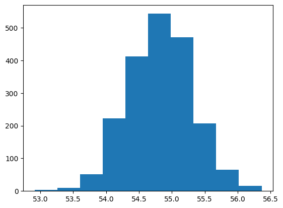
bootstrap distribution

mean_popularity_2000_boot = []

# Generate a bootstrap distribution of 2000 replicates
for i in range(2000):
    mean_popularity_2000_boot.append(
    	# Resample 500 rows and calculate the mean popularity     
    	spotify_sample["popularity"].sample(frac=1, replace=True).mean()
    )

# Print the bootstrap distribution results
plt.hist(mean_popularity_2000_boot)
plt.show()

# Calculate the population mean popularity
pop_mean = spotify_population["popularity"].mean()

# Calculate the original sample mean popularity
samp_mean = spotify_sample["popularity"].mean()

# Calculate the sampling dist'n estimate of mean popularity
samp_distn_mean = np.mean(mean_popularity_2000_samp)

# Calculate the bootstrap dist'n estimate of mean popularity
boot_distn_mean = np.mean(mean_popularity_2000_boot)

# Print the means
print([pop_mean, samp_mean, samp_distn_mean, boot_distn_mean])

[54.837142308430955, 54.8411, 54.824535000000004, 54.8397755]

dist_media_muestral = []

# Generate a sampling distribution of 2000 replicates
for i in range(2000):
    dist_media_muestral.append(
    	# Sample 500 rows and calculate the mean popularity 
    	coffee_ratings["flavor"].sample(n=500).mean()
    )

np.std(dist_media_muestral, ddof=1) * np.sqrt(500)

0.3169816193457466

# Population Standard deviation
coffee_ratings["flavor"].std(ddof=0)

0.3982932757401295

Confidence intervals

Confidence intervals define a range within the parameter or an statistic should be with a given certainty percentage.

Given a dataset, there are two ways of calculating confidence intervals (tipically 95%)

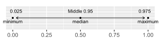
• Search from 2.5% to 97.5% of the dataset (Quantile method)

• Use the inverse of the cumulative density function and adjust it’s parameters (standard error method)

Quantile method for confidence intervals

To provide a 95% confidence interval for the normal distribution. We take the data contained within the 2.5 and 97.5 quantiles

Let’s do an example with the standard normal distribution.

# Generating a standard normal distribution

standard_normal = np.random.normal(0,1,1000000)

for the normal standard distribution:

np.quantile(standard_normal, 0.025)

-1.9557793224830742

for the normal standard distribution:

np.quantile(standard_normal, 0.975)

1.9647666250156202

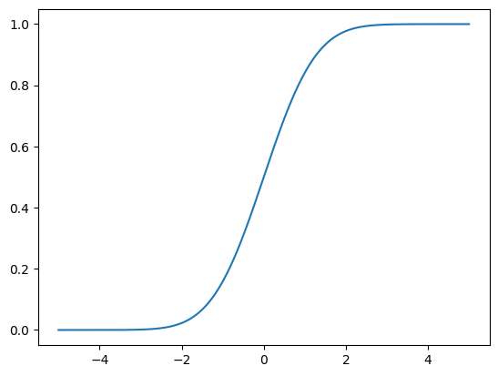
standard error method for confidence intervals

This method uses the Inverse Cumulative Distribution Function

First, let’s remember the Cumulative Distribution Function for a normal standard distribution

cumulative_density_function = []

for i in np.linspace(-5, 5, 1001):
    cumulative_density_function.append(norm.cdf(i, loc=0, scale=1))

plt.plot(np.linspace(-5, 5, 1001), cumulative_density_function)
plt.show()

Now, if you flip the x and y axis, you obtain the inverse of the cumulative density function

inverse_cumulative_density_function = []

for i in np.linspace(-5, 5, 1001):
    inverse_cumulative_density_function.append(norm.ppf(i, loc=0, scale=1))

plt.plot(np.linspace(-5, 5, 1001), inverse_cumulative_density_function)
plt.show()

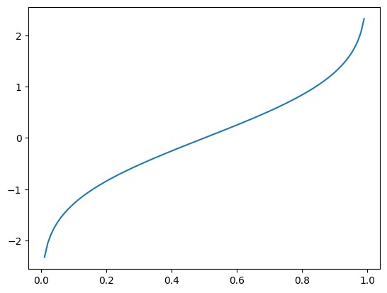
norm.ppf(0.025, loc= 0, scale=1)

-1.9599639845400545

the method consists of:

1. Calculate the point estimate: Which is the mean of the bootstrap distribution.

2. Calculate the standard error: Which is the standard deviation of the bootstrap distribution

3. Use the Inverse of the cumulative density function: Finally, call the norm.ppf() using the paramers

• the mean should be the point estimate of your distribution

• the standard deviation must be the standard error of your distribution

sources:

Datacamp: Sampling in python Platzi: Estadistica Inferencial

Hypotesis testing

Concept

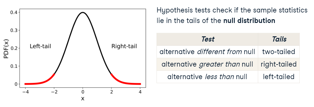
HYPOTHESIS TESTS DETERMINE WETHER THE SAMPLE STATISTICS LIE IN THE TAILS OF THE NULL DISTRIBUION

NULL DISTRIBUION: distribution of the statistic if the null hypothesis was true.

There are three types of tests. And the phrasing of the alternative hypothesis determines which type we should use

• If we are checking for a difference compared to a hypothesized value, we look for extreme values in either tail and perform a two-tailed test

• If the alternative hypothesis (\(H_1\)) uses language like “less” or “fewer”, we perform a left tailed test

• If the alternative hypothesis (\(H_1\)) uses language like “greater” or “exceeds”, correspond to a right tailed test

Assumptions

Every hypothesis has the following assumptions:

• each sample is randomly sourced from its population

this assumption exists because if the sample is not random, then it won’t be representative of the population

• each observation is independent

the only exception for this rule is the paired t-test (section 7) just because the data measures the same observation at a different time.

the fact than observations are dependent or independent change the calculations, not accounting for dependencies when they exist results in an increased chance of false negative or false positive error. Also, not accounting for dependencies is a problem hard to detect, and ideally needs to be discussed before data collection

to verify this assumption, you have to know your data source, there are no statistical tests to verify this assumption. The best way to onboard this problem is to ask people involved in the data collection, or a domain expert that understands the population being sampled.

• large sample size

These tests also assume that the sample is big enough that the central limit theorem applies and we can assume that the sample distribution is normal.

smaller samples incur greater uncertainty, implicating that central limith theorem does not apply and the sampling distributions might not be normally distributed

Also, the uncertainty generated by small sample means we get wider confidence intervals on the parameter we are trying to estimate

Now, How big our sample needs to be? depends on the test and will be shown across the upcoming chapters

• If the sample size is small In case of having small sample sizes not everything is lost, we can still work with them if the null distribution seems normal

Sanity check

One more check we can perform is to calcuate a bootstrap distribution and visualize it with a histogram, if we don’t see a bell shaped normal curve, then one of the assumptions hasn’t been met, in that case revisit the data collection process and check for

• randomness

• independence

• sample size

Hypothesis test (mean)

Steps to perform hypothesis testing

1. Define the null hypothesis and alternative hypothesis

2. Calculate the Z-score

since variables have arbitrary units and ranges, before we test our hypotesis, we need to standardize the values:

\(standardizedvalue = \frac{value - mean}{standard deviation}\)

But for hypotesis testing, we use a variation

z_score = \(\frac{sample statistic - hypoth.param.value}{standard error}\)

note:

sample statistic: is the statistic taken from your dataset or from the information you have

hypothesis parameter value: is the parameter that you define in your alternative hypothesis \(H_1\)

standard error: is the standard deviation of the bootstrap distribution

3. Calculate the P-value

Once you get the Z-score, you can now calculate the P-value. The calculation of the P-value depends on the test that you are performing

• for left-tailed test

p_value = norm.cdf(z_score, loc=0, scale=1)

• for right-tailed test

p_value = 1 - norm.cdf(z_score, loc=0, scale=1)

• for two-tailed test

p_value = 2 * norm.cdf(z_score, loc=0, scale=1)

• Note: norm.cdf() is a function of the scipy.stats library

to run it properly, run: from scipy.stats import norm

Finally, if the p-value is less than 0.05 (for a 0.05 significance level), you can reject the null hypothesis. Otherwise, you fail to reject the null hypothesis

Example1. TWO TAILED TEST

context

The dataset below contains information about the stack overflow yearly survey filtered to get answers only from people who consider theirselves as data scientist.

stack_overflow = pd.read_feather("stack_overflow.feather")

stack_overflow.head()

	respondent	main_branch	hobbyist	age	age_1st_code	age_first_code_cut	comp_freq	comp_total	converted_comp	country	...	survey_length	trans	undergrad_major	webframe_desire_next_year	webframe_worked_with	welcome_change	work_week_hrs	years_code	years_code_pro	age_cat
0	36.0	I am not primarily a developer, but I write co...	Yes	34.0	30.0	adult	Yearly	60000.0	77556.0	United Kingdom	...	Appropriate in length	No	Computer science, computer engineering, or sof...	Express;React.js	Express;React.js	Just as welcome now as I felt last year	40.0	4.0	3.0	At least 30
1	47.0	I am a developer by profession	Yes	53.0	10.0	child	Yearly	58000.0	74970.0	United Kingdom	...	Appropriate in length	No	A natural science (such as biology, chemistry,...	Flask;Spring	Flask;Spring	Just as welcome now as I felt last year	40.0	43.0	28.0	At least 30
2	69.0	I am a developer by profession	Yes	25.0	12.0	child	Yearly	550000.0	594539.0	France	...	Too short	No	Computer science, computer engineering, or sof...	Django;Flask	Django;Flask	Just as welcome now as I felt last year	40.0	13.0	3.0	Under 30
3	125.0	I am not primarily a developer, but I write co...	Yes	41.0	30.0	adult	Monthly	200000.0	2000000.0	United States	...	Appropriate in length	No	None	None	None	Just as welcome now as I felt last year	40.0	11.0	11.0	At least 30
4	147.0	I am not primarily a developer, but I write co...	No	28.0	15.0	adult	Yearly	50000.0	37816.0	Canada	...	Appropriate in length	No	Another engineering discipline (such as civil,...	None	Express;Flask	Just as welcome now as I felt last year	40.0	5.0	3.0	Under 30

5 rows × 63 columns

Let’s hypothesize that the mean anual compensation of the population of data scientists is 110.000 dollars

• \(H_0\) : The mean anual compensation of the population of data scientists is different from 110.000 dollars

• \(H_1\) : The mean anual compensation of the population of data scientists is 110.000 dollars

stack_overflow["converted_comp"].mean()

119574.71738168952

The result is different from our hypotesis, but, is it meaningfully different?

To answer that, we generate a bootstrap distribution of sample means

so_boot_distn = []

for i in range(5000):
    so_boot_distn.append(
        np.mean(
            stack_overflow.sample(frac=1, replace=True)["converted_comp"]
        )
    )

plt.hist(so_boot_distn, bins=50)
plt.show()

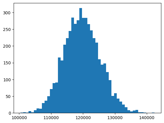
Notice that 110.000 is on the left of the distribution

Now, if we calculate the standard error (a.k.a standard deviation of the bootstrap distribution):

np.std(so_boot_distn, ddof=1)

5671.35937802767

since variables have arbitrary units and ranges, before we test our hypotesis, we need to standardize the values:

\(standardizedvalue = \frac{value - mean}{standard deviation}\)

But for hypotesis testing, we use a variation

\(z = \frac{sample statistic - hypoth.param.value}{standard error}\)

the result is called Z score

Calculating Z-score

z_score = ( stack_overflow["converted_comp"].mean() - 110000 ) / np.std(so_boot_distn, ddof=1)

z_score

1.6882579190422111

Calculating P-value

Since this is a two-tailed test, the pvalue is:

p_value = norm.cdf(z_score, loc=0, scale=1) * 2

p_value =  2 * ( 1 - norm.cdf(z_score, loc=0, scale=1) )

p_value

0.09136172933530817

And with this p-value and a significance level of 0.05, we failed to reject the null hypothesis and can conclude that the mean anual compensation of the population of data scientists is different from 110.000 dollars

Example2. RIGHT TAILED TEST

context

For this example, we will use the same dataframe of the stackoverflow survey for data scientists.

The variable age_first_code_cut classifies when Stack Overflow user first started programming

• “adult” means they started at 14 or older

• “child” means they started before 14

Let’s perform a hypothesis testing

• \(H_0\) : The proportion of data scientists starting programming as children is 35%

• \(H_1\) : The proportion of data scientists starting programming as children is greater than 35%

stack_overflow["age_first_code_cut"].head()

0    adult
1    child
2    child
3    adult
4    adult
Name: age_first_code_cut, dtype: object

We initially assume that the null hypothesis \(H_0\) is true. This only changes if the sample provides enough evidence to reject it.

Now let’s calculate the Zscore

Calculating Z score

# Point estimate
prop_child_samp = (stack_overflow["age_first_code_cut"] == "child").mean()
prop_child_samp

0.39141972578505085

# hypothesized statistic
prop_child_hyp = 0.35

# std_error
first_code_boot_distn = []

# bootstrap distribution
for i in range (5000):
    first_code_boot_distn.append(
        (stack_overflow.sample(frac=1, replace=True)["age_first_code_cut"] == "child").mean()
    )

std_error = np.std(first_code_boot_distn, ddof = 1)

std_error

0.0104640957859478

# Z-score

z_score = (prop_child_samp - prop_child_hyp) / std_error

z_score

3.958270894335017

Calculating P-value

Now, pass the z-score to the standard normal CDF (cumulative density function for standard normal distribution)

norm.cdf(z_score, loc=0, scale=1)

0.9999622528463471

And for final, as we are performing a right tail test, the P-value is calculated by taking

\(1 - norm.cdf()\)

p_value = 1 - norm.cdf(z_score, loc=0, scale=1)

p_value

3.77471536529006e-05

Therefore with a significance level of 0.05, we reject the null hypothesis and we can state that

The proportion of data scientists starting programming as children is greater than 35%

Example 3: RIGHT TAILED TEST

context

The late_shipments dataset contains supply chain data on the delivery of medical supplies. Each row represents one delivery of a part. The late columns denotes whether or not the part was delivered late.

late_shipments = pd.read_feather("late_shipments.feather")

late_shipments.head()

	id	country	managed_by	fulfill_via	vendor_inco_term	shipment_mode	late_delivery	late	product_group	sub_classification	...	line_item_quantity	line_item_value	pack_price	unit_price	manufacturing_site	first_line_designation	weight_kilograms	freight_cost_usd	freight_cost_groups	line_item_insurance_usd
0	36203.0	Nigeria	PMO - US	Direct Drop	EXW	Air	1.0	Yes	HRDT	HIV test	...	2996.0	266644.00	89.00	0.89	Alere Medical Co., Ltd.	Yes	1426.0	33279.83	expensive	373.83
1	30998.0	Botswana	PMO - US	Direct Drop	EXW	Air	0.0	No	HRDT	HIV test	...	25.0	800.00	32.00	1.60	Trinity Biotech, Plc	Yes	10.0	559.89	reasonable	1.72
2	69871.0	Vietnam	PMO - US	Direct Drop	EXW	Air	0.0	No	ARV	Adult	...	22925.0	110040.00	4.80	0.08	Hetero Unit III Hyderabad IN	Yes	3723.0	19056.13	expensive	181.57
3	17648.0	South Africa	PMO - US	Direct Drop	DDP	Ocean	0.0	No	ARV	Adult	...	152535.0	361507.95	2.37	0.04	Aurobindo Unit III, India	Yes	7698.0	11372.23	expensive	779.41
4	5647.0	Uganda	PMO - US	Direct Drop	EXW	Air	0.0	No	HRDT	HIV test - Ancillary	...	850.0	8.50	0.01	0.00	Inverness Japan	Yes	56.0	360.00	reasonable	0.01

5 rows × 27 columns

1. Calculate the proportion of late shipments

prop = (late_shipments["late"] == "Yes").mean()

prop

0.061

So, now we know that 0.061 or 6.1% of the sipments were late.

Let’s hipothesize that the proportion of late shipments is 6%

• \(H_0\): The proportion of late shipments is 6%

• \(H_1\): The proportion of late shipments is greater that 6%

and calculate a z score based on that hypothesis

Calculating Z score

late_shipments_boot_distn = []

# bootstrap distribution
for i in range (5000):
    late_shipments_boot_distn.append(
        (late_shipments.sample(frac=1, replace=True)["late"] == "Yes").mean()
    )

# standard error
std_error = np.std(late_shipments_boot_distn, ddof=1)

# remember: 
# z_score = (sample statistc - hypothesized statistic) / standard error

z_score = (prop - 0.06) / std_error

z_score

0.1318317224271221

And we got a z score of 0.13.

Now let’s calculate the pvalue

Calculating P-value

# Remember
# For right tailed test, p_value = 1 - norm.cdf(...)

p_value = 1 - norm.cdf(z_score, loc = 0, scale = 1)

p_value

0.4475586973291411

Since the P-value is greater that 0.05, at a significance level of 0.05, we failed to reject the null hypothesis and the conclusion is: The proportion of late shipments is not greater than 6%

Confirming the results with a confidence interval

Let’s calculate a confidence interval of 95%

# Calculate 95% confidence interval using quantile method
lower = np.quantile(late_shipments_boot_distn, 0.025)
upper = np.quantile(late_shipments_boot_distn, 0.975)

# Print the confidence interval
print((lower, upper))

(0.047, 0.076)

Note:

Since 0.06 is included in the 95% confidence interval and we failed to reject due to a large p-value, the results are similar.

Hypothesis test (difference of means)

Assumptions for sample size

These tests fall in the category of Two-sample t-tests, and we need at least 30 observations in each sample to fulfill the assumption

\(n_1 \geq 30, n_2 \geq 30\)

\(n_i\): sample size for group \(i\)

Example 1. Difference of means (right tailed)

Context

The dataset below contains information about the stack overflow yearly survey filtered to get answers only from people who consider theirselves as data scientist.

stack_overflow = pd.read_feather("stack_overflow.feather")

stack_overflow.head()

	respondent	main_branch	hobbyist	age	age_1st_code	age_first_code_cut	comp_freq	comp_total	converted_comp	country	...	survey_length	trans	undergrad_major	webframe_desire_next_year	webframe_worked_with	welcome_change	work_week_hrs	years_code	years_code_pro	age_cat
0	36.0	I am not primarily a developer, but I write co...	Yes	34.0	30.0	adult	Yearly	60000.0	77556.0	United Kingdom	...	Appropriate in length	No	Computer science, computer engineering, or sof...	Express;React.js	Express;React.js	Just as welcome now as I felt last year	40.0	4.0	3.0	At least 30
1	47.0	I am a developer by profession	Yes	53.0	10.0	child	Yearly	58000.0	74970.0	United Kingdom	...	Appropriate in length	No	A natural science (such as biology, chemistry,...	Flask;Spring	Flask;Spring	Just as welcome now as I felt last year	40.0	43.0	28.0	At least 30
2	69.0	I am a developer by profession	Yes	25.0	12.0	child	Yearly	550000.0	594539.0	France	...	Too short	No	Computer science, computer engineering, or sof...	Django;Flask	Django;Flask	Just as welcome now as I felt last year	40.0	13.0	3.0	Under 30
3	125.0	I am not primarily a developer, but I write co...	Yes	41.0	30.0	adult	Monthly	200000.0	2000000.0	United States	...	Appropriate in length	No	None	None	None	Just as welcome now as I felt last year	40.0	11.0	11.0	At least 30
4	147.0	I am not primarily a developer, but I write co...	No	28.0	15.0	adult	Yearly	50000.0	37816.0	Canada	...	Appropriate in length	No	Another engineering discipline (such as civil,...	None	Express;Flask	Just as welcome now as I felt last year	40.0	5.0	3.0	Under 30

5 rows × 63 columns

Two-sample problems compares sample statistics across groups of a variable

for the stack_overflow dataset:

• converted_comp is a numerical variable: describes mean salary in USD

• age_first_code_cut is a categorical value: describes if people started programming as childs or adults

The Hypothesis question is:

Are those users who first programmed as childs better compensated than those that started as adults?

\(H_0 : \) Population mean for both groups is the same \(H_1 : \) Population mean for those who started as childs is greater that for adults

\(H_0 : \mu_{child} - \mu_{adult} = 0 \)

\(H_1 : \mu_{child} - \mu_{adult} > 0 \)

Use a significance level of 0.05

stack_overflow.groupby("age_first_code_cut")["converted_comp"].mean()

age_first_code_cut
adult    111313.311047
child    132419.570621
Name: converted_comp, dtype: float64

The difference is notorius. But, is that increase statistically significant? or could it be explained by sampling variability?

Calculating T statistic

In this case, the test statistic for the hypothesis test is \(\bar{x}_{child} - \bar{x}_{adult}\), but in this case you don’t calculate the Z-score but the T stastictic

\(t = \frac{(\bar{x}_{child} - \bar{x}_{adult}) - (\mu_{child} - \mu_{adult})}{SE(\bar{x}_{child} - \bar{x}_{adult})} \)

and

\(SE(\bar{x}_{child} - \bar{x}_{adult}) \approx \sqrt{\frac{s^2_{child}}{n_{child}}+ \frac{s^2_{adult}}{n_{adult}}}\)

Now, since the null hypothesis assumes that the population means are equal, the final equation for t would be:

\(t = \frac{(\bar{x}_{child} - \bar{x}_{adult})}{\sqrt{\frac{s^2_{child}}{n_{child}}+ \frac{s^2_{adult}}{n_{adult}}}}\)

xbar = stack_overflow.groupby("age_first_code_cut")["converted_comp"].mean()
xbar_child = xbar[1]
xbar_adult = xbar[0]

s = stack_overflow.groupby("age_first_code_cut")["converted_comp"].std()
s_child = s[1]
s_adult = s[0]

n = stack_overflow.groupby("age_first_code_cut")["converted_comp"].count()
n_child = n[1]
n_adult = n[0]

numerator = xbar_child - xbar_adult

denominator = np.sqrt( ((s_child**2)/n_child) + ((s_adult**2)/n_adult ) )

t_stat = numerator/denominator

t_stat

1.8699313316221844

Calculating P value

The t distribution requests a degrees of freedom parameter (degrees of freedom are the amount of independant observations in our dataset).

In this case, there are as many degrees of freedom as observations, minus two, because we already know two sample statistics (the means for each group)

# dof = n - 2 
degrees_of_freedom = n_child + n_adult - 2

# since it is a right tailed test
P_value = 1 - t.cdf(t_stat, df=degrees_of_freedom)

P_value

0.030811302165157595

Since the P-value is less than 0.05, we reject the null hypothesis and can conclude that the mean salary for people who started coding as child, is higher than the mean salary for those who started as adults

Solving with pengouin

# Child compensation
child_compensation = stack_overflow[
    stack_overflow["age_first_code_cut"] == "child"]["converted_comp"]

# Adult compensation
adult_compensation = stack_overflow[
    stack_overflow["age_first_code_cut"] == "adult"]["converted_comp"]

pingouin.ttest(
    x = child_compensation,
    y = adult_compensation,
    alternative="greater"
)

	T	dof	alternative	p-val	CI95%	cohen-d	BF10	power
T-test	1.869931	1966.979249	greater	0.030821	[2531.75, inf]	0.079522	0.549	0.579301

Example 2. Difference of means (left tailed)

Context

The late_shipments dataset contains supply chain data on the delivery of medical supplies. Each row represents one delivery of a part. The late column denotes whether or not the part was delivered late.

late_shipments = pd.read_feather("late_shipments.feather")

late_shipments.head()

	id	country	managed_by	fulfill_via	vendor_inco_term	shipment_mode	late_delivery	late	product_group	sub_classification	...	line_item_quantity	line_item_value	pack_price	unit_price	manufacturing_site	first_line_designation	weight_kilograms	freight_cost_usd	freight_cost_groups	line_item_insurance_usd
0	36203.0	Nigeria	PMO - US	Direct Drop	EXW	Air	1.0	Yes	HRDT	HIV test	...	2996.0	266644.00	89.00	0.89	Alere Medical Co., Ltd.	Yes	1426.0	33279.83	expensive	373.83
1	30998.0	Botswana	PMO - US	Direct Drop	EXW	Air	0.0	No	HRDT	HIV test	...	25.0	800.00	32.00	1.60	Trinity Biotech, Plc	Yes	10.0	559.89	reasonable	1.72
2	69871.0	Vietnam	PMO - US	Direct Drop	EXW	Air	0.0	No	ARV	Adult	...	22925.0	110040.00	4.80	0.08	Hetero Unit III Hyderabad IN	Yes	3723.0	19056.13	expensive	181.57
3	17648.0	South Africa	PMO - US	Direct Drop	DDP	Ocean	0.0	No	ARV	Adult	...	152535.0	361507.95	2.37	0.04	Aurobindo Unit III, India	Yes	7698.0	11372.23	expensive	779.41
4	5647.0	Uganda	PMO - US	Direct Drop	EXW	Air	0.0	No	HRDT	HIV test - Ancillary	...	850.0	8.50	0.01	0.00	Inverness Japan	Yes	56.0	360.00	reasonable	0.01

5 rows × 27 columns

While trying to determine why some shipments are late, you may wonder if the weight of the shipments that were on time is less than the weight of the shipments that were late.

the weight_kilograms variable contains information about the weight of each shipment.

Then the hypothesis would be

\(H_0\): The mean weight of shipments that weren’t late is the same as the mean weight of shipments that were late. -> \(H_0: \mu_{late} = \mu_{on time}\) -> \(H_0: \mu_{late} - \mu_{on time} = 0\)

\(H_1\): The mean weight of shipments that weren’t late is less than the mean weight of shipments that were late. -> \(H_1: \mu_{on time} < \mu_{late} \) -> \(H_1: \mu_{on time} - \mu_{late} < 0\)

Calculating T statistic

xbar = late_shipments.groupby("late")["weight_kilograms"].mean()
xbar_no = xbar[0]
xbar_yes = xbar[1]

s = late_shipments.groupby("late")["weight_kilograms"].std()
s_no = s[0]
s_yes = s[1]

n = late_shipments.groupby("late")["weight_kilograms"].count()
n_no = n[0]
n_yes = n[1]

# Calculate the numerator of the test statistic
numerator = xbar_no - xbar_yes

# Calculate the denominator of the test statistic
denominator = np.sqrt( ((s_no**2)/n_no) + ((s_yes**2)/n_yes) )

# Calculate the test statistic
t_stat = numerator/denominator

t_stat

-2.3936661778766433

Calculating P-value

# Calculate the degrees of freedom
degrees_of_freedom = n_no + n_yes - 2

# Calculate the p-value from the test stat
p_value = t.cdf(t_stat, df = degrees_of_freedom)

p_value

0.008432382146249523

In fact, we can now reject the null hypothesis and conclude that the mean weight for those shipments that were delivered late is higher

Hypothesis testing (paired data)

Assumptions for sample size

This tests falls into the category of paired-sample t-tests and the assumptions for this category are that we have at least 30 pairs of observations across the samples

No. of rows in our data \(\geq 30\)

Example 1. Difference of means (left tailed)

Context

The dataset below, refers to the results for republicans in 2008 and 2012 presidential elections, each row represents a republicans result for presidential elections at a county level

republicans = pd.read_feather("repub_votes_potus_08_12.feather")

republicans

	state	county	repub_percent_08	repub_percent_12	diff
0	Alabama	Hale	38.957877	37.139882	1.817995
1	Arkansas	Nevada	56.726272	58.983452	-2.257179
2	California	Lake	38.896719	39.331367	-0.434648
3	California	Ventura	42.923190	45.250693	-2.327503
4	Colorado	Lincoln	74.522569	73.764757	0.757812
...	...	...	...	...	...
95	Wisconsin	Burnett	48.342541	52.437478	-4.094937
96	Wisconsin	La Crosse	37.490904	40.577038	-3.086134
97	Wisconsin	Lafayette	38.104967	41.675050	-3.570083
98	Wyoming	Weston	76.684241	83.983328	-7.299087
99	Alaska	District 34	77.063259	40.789626	36.273633

100 rows × 5 columns

Given this dataset, the question is:

Was the percentage of republican candidate votes lower in 2008 than in 2012?

\(H_{0}: \mu_{2008} - \mu_{2012} = 0\)

\(H_{1}: \mu_{2008} - \mu_{2012} < 0\)

let´s use a significance level of 0.05

One detail of this dataset is that 2008 and 2012 votes are paired meaning they are not independant

and we want to capture voting patterns in the model

now, for paired analysis, rather than considering the two variables separatedly, we can consider a single variable of the difference. Let´s store that difference in a dataframe called sample_data and the variable called diff

sample_data = republicans

sample_data["diff"] = sample_data["repub_percent_08"] - sample_data["repub_percent_12"]

sample_data["diff"].hist(bins=20)

<AxesSubplot: >

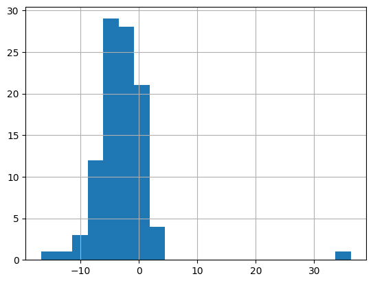
in the histogram, you can notice that most values are between -10 and 0, including an outlier

now let´s calculate the sample mean

xbar_diff = sample_data["diff"].mean()

xbar_diff

-2.877109041242944

now, we can restate the hypothesis in terms of \(\mu_{diff}\)

\(H_{0}: \mu_{diff} = 0\)

\(H_{1}: \mu_{diff} < 0\)

Calculating T statistic

the t statistic in this case has a slightly variation, the equation in this case would be

\(t = \frac{\bar{x}_{diff} - \mu_{diff}}{\sqrt{\frac{s^2_{diff}}{n_{diff}}}}\)

and also, in this case we know one statistic. Then, the numbers of degrees of freedoms would be the number of records minus one

dof = ndiff - 1

# calculating t

n_diff = len(sample_data)

s_diff = sample_data["diff"].std()

t_stat = (xbar_diff - 0)/np.sqrt((s_diff**2)/n_diff)

t_stat

-5.601043121928489

Calculating P value

p_value = t.cdf(t_stat, df = n_diff-1)

p_value

9.572537285272411e-08

This means we can reject the null hypothesis and can conclude that the percentage of votes for republicans was lower in 2008 compared to 2012.

solving with pingouin

The pingouin package provides methods for hypothesis testing and provides an output as a pandas dataframe.

The method that we will use is ttest

• The first argument is the series of differences

• The argument y specifies the hypothesized difference value from the null hypothesis (in this case is zero)

• The alternative hypothesis can be specified as “two-sided” for two tailed tests, “less” for left tailed tests or “greater” for right tailed tests

pingouin.ttest(
    x = sample_data["diff"],
    y = 0,
    alternative = "less"
)

	T	dof	alternative	p-val	CI95%	cohen-d	BF10	power
T-test	-5.601043	99	less	9.572537e-08	[-inf, -2.02]	0.560104	1.323e+05	1.0

And you can see that the result is the same, null hypothesis is rejected

pingouin variation of t-test for paired data

pingouin offers a variation that requires even less work, which is useful for paired data

pingouin.ttest(
    x = sample_data["repub_percent_08"],
    y = sample_data["repub_percent_12"],
    paired = True,    #this argument is very important for paired data
    alternative="less"
)

	T	dof	alternative	p-val	CI95%	cohen-d	BF10	power
T-test	-5.601043	99	less	9.572537e-08	[-inf, -2.02]	0.217364	1.323e+05	0.696338

Example 2. Difference of means (two-tailed)

Context

The dataset below, refers to the results for democrats in 2012 and 2016 presidential elections, each row represents democrats result for presidential elections at a county level

democrats = pd.read_feather("dem_votes_potus_12_16.feather")

democrats.head()

	state	county	dem_percent_12	dem_percent_16
0	Alabama	Bullock	76.305900	74.946921
1	Alabama	Chilton	19.453671	15.847352
2	Alabama	Clay	26.673672	18.674517
3	Alabama	Cullman	14.661752	10.028252
4	Alabama	Escambia	36.915731	31.020546

You’ll explore the difference between the proportion of county-level votes for the Democratic candidate in 2012 and 2016 to identify if the difference is significant. The hypotheses are as follows:

\(H_0\) : The proportion of democratic votes in 2012 and 2016 were the same. \(H_1\) : The proportion of democratic votes in 2012 and 2016 were different.

Solving with pingouin

pingouin.ttest(
    x = democrats['dem_percent_12'],
    y = democrats['dem_percent_16'],
    paired = True,
    alternative = "two-sided"
)

	T	dof	alternative	p-val	CI95%	cohen-d	BF10	power
T-test	30.298384	499	two-sided	3.600634e-115	[6.39, 7.27]	0.454202	2.246e+111	1.0

then, you can reject the null hypothesis

Hypothesis test (ANOVA)

Assumptions for sample size

Since ANOVA compares a numerical value across multiple categories (three or more), we need at least 30 observations in each sample to fulfill the assumption

\(n_i \geq 30\) for all values of \(i\)

When to use ANOVA

ANOVA tests are used when you want to compare the behavior of a numerical variable between three or more groups

let’s analyze two variables from the stack_overflow dataset

• job_sat: describes how satisfied are people with their jobs

• converted_comp shows compensation in USD

stack_overflow = pd.read_feather("stack_overflow.feather")

stack_overflow[["job_sat", "converted_comp"]].head()

	job_sat	converted_comp
0	Slightly satisfied	77556.0
1	Very satisfied	74970.0
2	Very satisfied	594539.0
3	Very satisfied	2000000.0
4	Very satisfied	37816.0

A hypothesis question could be:

Is compensation different across the levels of satisfaction?

The first step is to visualize it in a boxplot

sns.boxplot(
    x = stack_overflow["converted_comp"],
    y = stack_overflow["job_sat"],
    data = stack_overflow
)

plt.show()

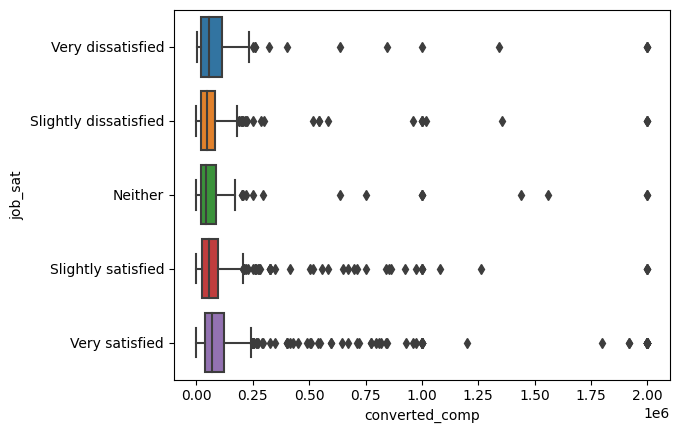
And it looks nice, but let’s remove the outliers to see the distribution better

sns.boxplot(
    x = stack_overflow["converted_comp"],
    y = stack_overflow["job_sat"],
    data = stack_overflow,
    showfliers = False
)

plt.show()

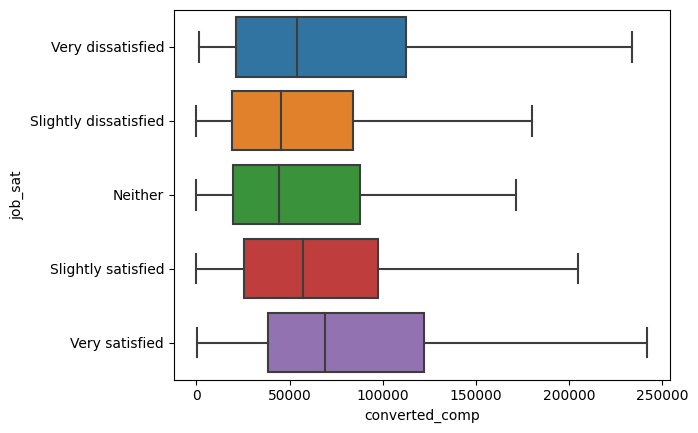
And looks like there are differences, but are these statistically significant?

Let’s test it using the pingouin.anova method, using a significance level of 0.2

pingouin.anova() method

pingouin.anova(
    data = stack_overflow,
    dv = "converted_comp",              #Dependant Variable
    between= "job_sat"
)

	Source	ddof1	ddof2	F	p-unc	np2
0	job_sat	4	2256	4.480485	0.001315	0.007882

This p-value is 0.0013, which is less than 0.2, that indicates that at least two categories of job satisfaction have significant differences between their compensation levels

BUT THIS DOESN’T TELL US WHICH TWO CATEGORIES THEY ARE

to identify which categories are different, you have to compare all the categories as shown below:

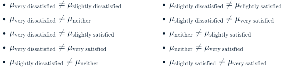
pairwise tests

To do this, let’s use a pairwise test

notice that the three first arguments are the same as ANOVA test, we will discuss the p-adjust shortly

pingouin.pairwise_tests(
    data = stack_overflow,
    dv = "converted_comp",
    between= "job_sat",
    padjust= "none"
)

	Contrast	A	B	Paired	Parametric	T	dof	alternative	p-unc	BF10	hedges
0	job_sat	Slightly satisfied	Very satisfied	False	True	-4.009935	1478.622799	two-sided	0.000064	158.564	-0.192931
1	job_sat	Slightly satisfied	Neither	False	True	-0.700752	258.204546	two-sided	0.484088	0.114	-0.068513
2	job_sat	Slightly satisfied	Very dissatisfied	False	True	-1.243665	187.153329	two-sided	0.215179	0.208	-0.145624
3	job_sat	Slightly satisfied	Slightly dissatisfied	False	True	-0.038264	569.926329	two-sided	0.969491	0.074	-0.002719
4	job_sat	Very satisfied	Neither	False	True	1.662901	328.326639	two-sided	0.097286	0.337	0.120115
5	job_sat	Very satisfied	Very dissatisfied	False	True	0.747379	221.666205	two-sided	0.455627	0.126	0.063479
6	job_sat	Very satisfied	Slightly dissatisfied	False	True	3.076222	821.303063	two-sided	0.002166	7.43	0.173247
7	job_sat	Neither	Very dissatisfied	False	True	-0.545948	321.165726	two-sided	0.585481	0.135	-0.058537
8	job_sat	Neither	Slightly dissatisfied	False	True	0.602209	367.730081	two-sided	0.547406	0.118	0.055707
9	job_sat	Very dissatisfied	Slightly dissatisfied	False	True	1.129951	247.570187	two-sided	0.259590	0.197	0.119131

If we analyze the output, in the p-unc column, we will notice that three of them are less than our significance level of 0.2

Note that for pairwise tests, as the number of groups increase, the number of pairs increase cuadratically (in this case we got 10 pairs out of 5 groups)

false positive danger

And if the pairs increases cuadratically, the number of hypothesis tests we must perform increases cuadratically.

Now, performing a lot of hypothesis tests increase the probability of getting a false positive significant result, the chart below shows the probability of a false positive vs the amount of hypothesis tests ran

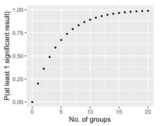
Note that:

• with a significance level of 0.2, running one test, the probability of a false positive is approximately 0.2!

• with 5 groups (which means 10 tests), the probability of false positive is around 0.7!

• with 20 groups, it’s almost guaranteed that you will have at least one false positive!

The solution to this problem

The solution for this problem of getting a false positive is to apply an adjustment to increase the p-values (and therefore reducing the probability of false positive)

• one common adjustment is the bonferroni correction

p -value adjustment (bonferroni)

pingouin.pairwise_tests(
    data = stack_overflow,
    dv = "converted_comp",
    between= "job_sat",
    padjust= "bonf"
)

	Contrast	A	B	Paired	Parametric	T	dof	alternative	p-unc	p-corr	p-adjust	BF10	hedges
0	job_sat	Slightly satisfied	Very satisfied	False	True	-4.009935	1478.622799	two-sided	0.000064	0.000638	bonf	158.564	-0.192931
1	job_sat	Slightly satisfied	Neither	False	True	-0.700752	258.204546	two-sided	0.484088	1.000000	bonf	0.114	-0.068513
2	job_sat	Slightly satisfied	Very dissatisfied	False	True	-1.243665	187.153329	two-sided	0.215179	1.000000	bonf	0.208	-0.145624
3	job_sat	Slightly satisfied	Slightly dissatisfied	False	True	-0.038264	569.926329	two-sided	0.969491	1.000000	bonf	0.074	-0.002719
4	job_sat	Very satisfied	Neither	False	True	1.662901	328.326639	two-sided	0.097286	0.972864	bonf	0.337	0.120115
5	job_sat	Very satisfied	Very dissatisfied	False	True	0.747379	221.666205	two-sided	0.455627	1.000000	bonf	0.126	0.063479
6	job_sat	Very satisfied	Slightly dissatisfied	False	True	3.076222	821.303063	two-sided	0.002166	0.021659	bonf	7.43	0.173247
7	job_sat	Neither	Very dissatisfied	False	True	-0.545948	321.165726	two-sided	0.585481	1.000000	bonf	0.135	-0.058537
8	job_sat	Neither	Slightly dissatisfied	False	True	0.602209	367.730081	two-sided	0.547406	1.000000	bonf	0.118	0.055707
9	job_sat	Very dissatisfied	Slightly dissatisfied	False	True	1.129951	247.570187	two-sided	0.259590	1.000000	bonf	0.197	0.119131

Now, if we analyze the p-corr column, which is the adjusted p-value, we will note that only two of the pairs have an statistically significant difference

Great! p-value adjustment is the solution for when you have a ton of pairs!

pingouin offers many other options for adjusting the p-values, some are more conservative than others.

Example 2 ANOVA (three categories)

Given the late shipments data, let’s analyze how the price of each package (pack_price) varies between the three shipment modes (shipment_mode): “Air”, “Air Charter”, and “Ocean”.

late_shipments = pd.read_feather("late_shipments.feather")

late_shipments[["shipment_mode", "pack_price"]].head()

	shipment_mode	pack_price
0	Air	89.00
1	Air	32.00
2	Air	4.80
3	Ocean	2.37
4	Air	0.01

\(H_0\): Pack prices for every category of shipment mode are the same.

\(H_1\): Pack prices for some categories of shipment mode are different.

\(\alpha = 0.1\)

Checking sample size assumptions

# Count the shipment_mode values
counts = late_shipments["shipment_mode"].value_counts()

# Print the result
print(counts)

# Inspect whether the counts are big enough
print((counts >= 30).all())

Air            905
Ocean           88
Air Charter      6
Name: shipment_mode, dtype: int64
False

The assumptions are not met for that Air Charter category, therefore, we should be a little cautious of the results given that small sample size.

Exploratory Data Analysis per Group

let’s explore first with the average price for each group

late_shipments.groupby("shipment_mode")["pack_price"].mean()

shipment_mode
Air            39.712395
Air Charter     4.226667
Ocean           6.432273
Name: pack_price, dtype: float64

Looks like the air is way more expensive than the other two categories

let’s see the dispersion as well:

late_shipments.groupby("shipment_mode")['pack_price'].std()

shipment_mode
Air            48.932861
Air Charter     0.992969
Ocean           5.303047
Name: pack_price, dtype: float64

data for “air” is more dispersed

Now let’s see the boxplots:

sns.boxplot(
    x = late_shipments["pack_price"],
    y = late_shipments["shipment_mode"],
    data = late_shipments
)
plt.show()

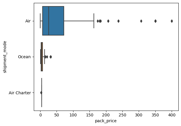
Great, now let’s see if this difference statistically significant

Conducting ANOVA

pingouin.anova(
    data = late_shipments,
    dv = "pack_price",              #Dependant Variable
    between= "shipment_mode"
)

	Source	ddof1	ddof2	F	p-unc	np2
0	shipment_mode	2	997	21.8646	5.089479e-10	0.042018

the p-unc (p value) indicates that there is difference between at least one pair, let’s perform pairwise tests to confirm which pairs are these

Pairwise tests

pingouin.pairwise_tests(
    data = late_shipments,
    dv = "pack_price",
    between = "shipment_mode"
)

	Contrast	A	B	Paired	Parametric	T	dof	alternative	p-unc	BF10	hedges
0	shipment_mode	Air	Air Charter	False	True	21.179625	600.685682	two-sided	8.748346e-75	5.809e+76	0.726592
1	shipment_mode	Air	Ocean	False	True	19.335760	986.979785	two-sided	6.934555e-71	1.129e+67	0.711119
2	shipment_mode	Air Charter	Ocean	False	True	-3.170654	35.615026	two-sided	3.123012e-03	15.277	-0.423775

without adjustment, the p value in each test indicates that there is a significant difference between all the pairs, let’s see the results again with the adjustment

P-value adjustment (bonferroni)

pingouin.pairwise_tests(
    data = late_shipments,
    dv = "pack_price",
    between = "shipment_mode",
    padjust = "bonf"
)

	Contrast	A	B	Paired	Parametric	T	dof	alternative	p-unc	p-corr	p-adjust	BF10	hedges
0	shipment_mode	Air	Air Charter	False	True	21.179625	600.685682	two-sided	8.748346e-75	2.624504e-74	bonf	5.809e+76	0.726592
1	shipment_mode	Air	Ocean	False	True	19.335760	986.979785	two-sided	6.934555e-71	2.080367e-70	bonf	1.129e+67	0.711119
2	shipment_mode	Air Charter	Ocean	False	True	-3.170654	35.615026	two-sided	3.123012e-03	9.369037e-03	bonf	15.277	-0.423775

adjusted p-value shows similar results, all the p-values are smaller than 0.1!

then we can conclude:

for the pairs below, we can reject the null hypothesis that the pack prices are equal:

• \(\mu_{air} > \mu_{air-charter}\)

• \(\mu_{air} > \mu_{ocean}\)

• \(\mu_{ocean} >\mu_{air-charter}\)

Hypothesis test (tests for proportions)

when you refer to hypothesis tests for proportions,

\(p\) is the population proportion (unknown parameter)

\(\hat{p}\) is the sample proportion (sample statistic)

\(p_0\) is the hypothesized population proportion

Now, when performing the hypothesis testing, the test statistic is:

\(z = \frac{\hat{p} - p_0}{\sqrt{\frac{p_0 * (1 - p_0)}{n}}}\)

Assumptions for sample size

Since this is a one-sample proportion test, the number of successes and the number of failures in sample is greater than or equal to 10

\(n * \hat{p} \geq 10\)

\(n * (1 - \hat{p}) \geq 10\)

\(n\): sample size \(\hat{p}\): proportion of successes in sample

Example 1 (two-tailed test)

Context

Returning to the stack overflow survey, let’s hypothesize that half of the users are under thirty

\(H_0\) : Proportions of stackoverflow users under thirty = 0.5

\(H_1\) : Proportions of stackoverflow users under thirty \(\neq\) 0.5

\(\alpha\) = 0.01

let’s check the sample first

stack_overflow["age_cat"].value_counts(normalize = True)

Under 30       0.535604
At least 30    0.464396
Name: age_cat, dtype: float64

given this information, let’s check our hypothesis

Calculate z score

p_hat = (stack_overflow["age_cat"] == "Under 30").mean()

p_0 = 0.5

n = len(stack_overflow)

z_score = (p_hat - p_0) / np.sqrt( (p_0 * (1 - p_0))/ n )

z_score

3.385911440783663

Calculating p-value

#substract from 1 since p-value is positive
p_value = 2 * (1 - norm.cdf(z_score)) 

p_value

0.0007094227368100725

Since the p_value is less than the alpha, then we can reject the null hypothesis

Example 2 (right tailed test)

Given the late shipments dataset, let’s Hypothesize that the proportion of late shipments is greater than 6%.

H_0 = proportion of late shipments is 6%.

H_1 = proportion of late shipments is greater than 6%.

late_shipments = pd.read_feather("late_shipments.feather")

Checking for sample size assumptions

# Count the late values
counts = late_shipments["late"].value_counts()

# Print the result
print(counts)

# Inspect whether the counts are big enough
print((counts >= 10).all())

No     939
Yes     61
Name: late, dtype: int64
True

Since there are more than 10 successes and failures, assumptions are fulfilled

Calculating z-score

# Hypothesize that the proportion of late shipments is 6%
p_0 = 0.06

# Calculate the sample proportion of late shipments
p_hat = (late_shipments['late'] == "Yes").mean()

# Calculate the sample size
n = len(late_shipments)

# Calculate the numerator and denominator of the test statistic
numerator = p_hat - p_0
denominator = np.sqrt(p_0 * (1 - p_0) / n)

# Calculate the test statistic
z_score = numerator / denominator

Calculating p-value

# Calculate the p-value from the z-score
p_value = 1 - norm.cdf(z_score)

# Print the p-value
print(p_value)

0.44703503936503364

then, we failed to reject the null hypothesis

Hypothesis test (tests for differences of proportions)

Assumptions for sample size

Since this is a two-sample proportion test, the number of successes and the number of failures in each sample is greater than or equal to 10

\(n_1 * \hat{p}_1 \geq 10\) \(n_2 * \hat{p}_2 \geq 10\)

\(n_1 * (1 - \hat{p}_1) \geq 10\) \(n_2 * (1 - \hat{p}_2) \geq 10\)

\(n\): sample size \(\hat{p}\): proportion of successes in sample

Example 1 (two-tailed)

Context

In the stack overflow dataset, there is a variable called hobbyist

the value “yes” indicates that the users considers themselves as a hobbyist and “no” indicates that they consider themselves as professionals

\(H_0\): proportion of hobbyist users is the same for those under thirty as those at leats thirty \(H_0\): \(p_{\geq 30} - p_{< 30} = 0 \)

\(H_1\): proportion of hobbyist users is different for those unnder thirty as those at leats thirty \(H_0\): \(p_{\geq 30} - p_{< 30} \neq 0 \)

\(\alpha\) = 0.05

exploring the proportions between the age categories, we get:

stack_overflow.groupby("age_cat")["hobbyist"].value_counts(normalize = True)

age_cat      hobbyist
At least 30  Yes         0.773333
             No          0.226667
Under 30     Yes         0.843105
             No          0.156895
Name: hobbyist, dtype: float64

but, is it statistically significant?

Calculating the Z score

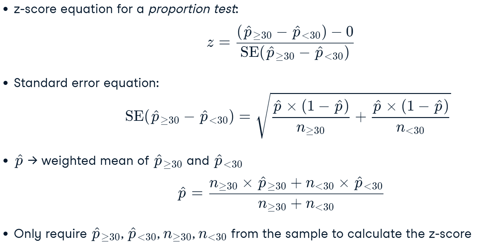
p_hats = stack_overflow.groupby("age_cat")["hobbyist"].value_counts(normalize = True)

p_hats

age_cat      hobbyist
At least 30  Yes         0.773333
             No          0.226667
Under 30     Yes         0.843105
             No          0.156895
Name: hobbyist, dtype: float64

p_hat_at_least_30 = p_hats[("At least 30", "Yes")]

p_hat_under_30 = p_hats[("Under 30", "Yes")]

print(p_hat_at_least_30, p_hat_under_30)

0.7733333333333333 0.8431048720066061

n = stack_overflow.groupby("age_cat")["hobbyist"].count()

n

age_cat
At least 30    1050
Under 30       1211
Name: hobbyist, dtype: int64

n_at_least_30 = n["At least 30"]

n_under_30 = n["Under 30"]

print(n_at_least_30, n_under_30)

1050 1211

# calculating p_hat

p_hat = (
    (n_at_least_30 * p_hat_at_least_30 + n_under_30 * p_hat_under_30)/
    (n_at_least_30 + n_under_30)
)

# calculating standard error
std_error = np.sqrt(p_hat * (1 - p_hat) / n_at_least_30 + 
                    p_hat * (1 - p_hat) / n_under_30)

# calculating z-score
z_score = (p_hat_at_least_30 - p_hat_under_30) / std_error
z_score

-4.223691463320559

Calculating p-value

# p-value for two sided test
2 * norm.cdf(z_score)

2.403330142685068e-05

Therefore, we can reject the null hypothesis

Calculating with statsmodels

This function requires two arguments:

• the number of hobbyists in each category

• the total number of rows in each group

stack_overflow.groupby("age_cat")["hobbyist"].value_counts()

age_cat      hobbyist
At least 30  Yes          812
             No           238
Under 30     Yes         1021
             No           190
Name: hobbyist, dtype: int64

n_hobbyists = np.array([812, 1021])

n_hobbyists

array([ 812, 1021])

n_rows = np.array([812 + 238, 1021 + 190])

n_rows

array([1050, 1211])

from statsmodels.stats.proportion import proportions_ztest

z_score, p_value = proportions_ztest(count=n_hobbyists,
 nobs=n_rows, alternative="two-sided")

print(z_score, p_value)

-4.223691463320559 2.403330142685068e-05

the p-value is smaller than our alpha, meaning that we can reject the null hypothesis

Example 2 (right tailed)

Context

You may wonder if the amount paid for freight affects whether or not the shipment was late. Recall that in the late_shipments dataset, whether or not the shipment was late is stored in the late column. Freight costs are stored in the freight_cost_group column, and the categories are “expensive” and “reasonable”

The hypotheses to test, with “late” corresponding to the proportion of late shipments for that group, are

\(H_{0}: late_{expensive} - late_{reasonable} = 0\) \(H_{1}: late_{expensive} - late_{reasonable} > 0\)

p_hats = (
    late_shipments.
    groupby("freight_cost_groups")["late"].value_counts(normalize=True)
).filter(like='Yes', axis=0)

p_hats

freight_cost_groups  late
expensive            Yes     0.079096
reasonable           Yes     0.035165
Name: late, dtype: float64

# sample size
ns = late_shipments.groupby("freight_cost_groups")["late"].count()

ns

freight_cost_groups
expensive     531
reasonable    455
Name: late, dtype: int64

Now that we have the p hats and the n, let’s calculate the p-hat

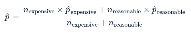
p_hat = (
    (p_hats["reasonable"] * ns["reasonable"] +
     p_hats["expensive"] * ns["expensive"]) / 
    (ns["reasonable"] + ns["expensive"])
)

p_hat

late
Yes    0.058824
Name: late, dtype: float64

now that we have the p_hat, let’s calculate the standard error of the sample as follows:

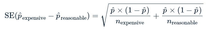
# Calculate the standard error
std_error = np.sqrt(
    ( ( p_hat * (1 - p_hat) ) / ns["expensive"] )+
    ( ( p_hat * (1 - p_hat) ) / ns["reasonable"] )
)

std_error

late
Yes    0.015031
Name: late, dtype: float64

Calculating Z score

z_score = (p_hats["expensive"] - p_hats["reasonable"])/std_error

z_score

late
Yes    2.922649
Name: late, dtype: float64

Calculating p value

# Right tailed test
p_value = 1 - norm.cdf(z_score)

p_value

array([0.00173534])

With this p-value we can reject the null hypothesis and conclude that the proportion of late deliveries for expensive-priced shipments is greater than the proportion for reasonable-priced shipments

Calculating with statmodels

# Count the late column values for each freight_cost_group
late_by_freight_cost_group = (
    late_shipments.groupby("freight_cost_groups")["late"].value_counts()
)

success_counts

freight_cost_groups  late
expensive            No      489
                     Yes      42
reasonable           No      439
                     Yes      16
Name: late, dtype: int64

success_counts = np.array(
    [
        late_by_freight_cost_group[("expensive","Yes")],
        late_by_freight_cost_group[("reasonable","Yes")]
    ]
)

success_counts

array([42, 16])

n = np.array([
    late_by_freight_cost_group["expensive"].sum(),
    late_by_freight_cost_group["reasonable"].sum()
    ])

n

array([531, 455])

stat, p_value = proportions_ztest(
    count = success_counts,
    nobs = n,
    alternative = "larger"

)

print(stat, p_value)

2.922648567784529 0.001735340002359578

And we got the same results, same p-value!

Chi Squared Tests of independance

Assumptions for sample size

The number of successes and failures in each group is greater that or equal to 5

\(n_1 * \hat{p}_i \geq 5\)

\(n_1 * (1 - \hat{p}_i) \geq 5\)

\(n_i\): sample size for group \(i\)

\(\hat{p}\): proportion of successes in sample group \(i\)

Example 1

This test measures the independance between two categorical variables

Two categorical variables are statistically independant when the proportion of successes in the response variable is the same across all the categories of the explanatory variable

let’s use the pingouin package to determine if the “hobbyist” and “age_cat” variables from the stack_overflow survey datasetare independant

\(H_0 :\) Age categories are independent of hobbyist autoperception \(H_1 :\) Age categories are not independent of hobbyist autoperception

props = (
    stack_overflow
    .groupby("hobbyist")["age_cat"]
    .value_counts(normalize = True)
)

wide_props = props.unstack()

wide_props.plot(kind = "bar", stacked = True)

<AxesSubplot: xlabel='hobbyist'>

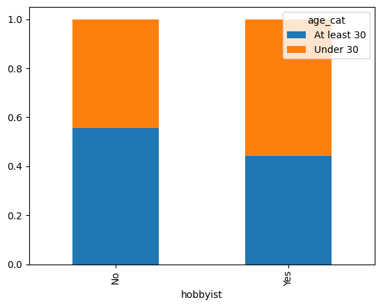
This chart may suggest that the variables are not indepentant, because looks like the proportion of hobbyists is higher in people under 30.

Let’s confirm if these variables are statistically independant

Calculating degrees of freedom

in this case, there are two categorical variables with two categories each, then the degrees of freedom are calculated:

\(dof =\) (No. of response categories - 1) x (No. of explanatory categories - 1) \(dof = (2-1)*(2-1) = 1\)

Yates’ continuity correction

Is a correction only applied when the sample size is very small and the degrees of freedom is one. Carefull!, the only way to apply it is if \(dof = 1\), otherwise, it won’t be applied by default

In this case, since each group has over 1000 observations, we don’t need it here

expected, observed, stats = pingouin.chi2_independence(
    data = stack_overflow,
    x = "hobbyist",
    y = "age_cat",
    correction= False
)

stats

	test	lambda	chi2	dof	pval	cramer	power
0	pearson	1.000000	17.387820	1.0	0.000030	0.087694	0.986444
1	cressie-read	0.666667	17.366950	1.0	0.000031	0.087642	0.986357
2	log-likelihood	0.000000	17.351288	1.0	0.000031	0.087602	0.986291
3	freeman-tukey	-0.500000	17.362338	1.0	0.000031	0.087630	0.986338
4	mod-log-likelihood	-1.000000	17.392980	1.0	0.000030	0.087707	0.986466
5	neyman	-2.000000	17.513563	1.0	0.000029	0.088011	0.986958

This extremely low value for p value suggests that the variables are not independent since the null hypothesis has been rejected

Example 2

The stack overflow dataset contains a variable called job_sat which measures job satisfaction and another called age_cat which says if people is under 30 or not.

stack_overflow["age_cat"].value_counts()

Under 30       1211
At least 30    1050
Name: age_cat, dtype: int64

stack_overflow["job_sat"].value_counts()

Very satisfied           879
Slightly satisfied       680
Slightly dissatisfied    342
Neither                  201
Very dissatisfied        159
Name: job_sat, dtype: int64

\(H_0 :\) Age categories are independent of job satisfaction levels \(H_1 :\) Age categories are not independent of job satisfaction levels

\(\alpha = 0.1\)

btw age category is the response variable and job satisfaction is the explanatory variable

props = (
    stack_overflow
    .groupby("job_sat")["age_cat"]
    .value_counts(normalize = True)
)

wide_props = props.unstack()

wide_props.plot(kind = "bar", stacked = True)

<AxesSubplot: xlabel='job_sat'>

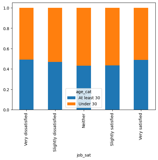
From this chart we may think:

• if the proportions are too close in each category the variables are independent

• if the proportions are too different, the variables are not independent

this chart suggests that the difference is not that big, and we may consider that variables are independent

In this case, we have to perform the chi-squared test to see if the variables are statistically independent

Calculate degrees of freedom

in this case, there are two categorical variables with two categories each, then the degrees of freedom are calculated:

\(dof =\) (No. of response categories - 1) x (No. of explanatory categories - 1) \(dof = (2-1)*(5-1) = 4\)

Since we have 4 dof, we don’t care about yate’s correction, it is only applied by default when dof = 1.

expected, observed, stats = pingouin.chi2_independence(
    data = stack_overflow,
    x = "job_sat",
    y = "age_cat",
    correction= False
)

stats

	test	lambda	chi2	dof	pval	cramer	power
0	pearson	1.000000	5.552373	4.0	0.235164	0.049555	0.437417
1	cressie-read	0.666667	5.554106	4.0	0.235014	0.049563	0.437545
2	log-likelihood	0.000000	5.558529	4.0	0.234632	0.049583	0.437871
3	freeman-tukey	-0.500000	5.562688	4.0	0.234274	0.049601	0.438178
4	mod-log-likelihood	-1.000000	5.567570	4.0	0.233854	0.049623	0.438538
5	neyman	-2.000000	5.579519	4.0	0.232828	0.049676	0.439419

Since p value is not smaller than \(\alpha\), we failed to reject \(H_0\) and yes, variables are independent!

Example 3

In the late_shipments dataset, there is a variable called vendor_inco_term that describes the incoterms applied to a shipment

incoterms: Trade deals often use a form of business shorthand in order to specify the exact details of their contract. These are International Chamber of Commerce (ICC) international commercial terms, or incoterms for short.

The options are:

EXW: “Ex works”. The buyer pays for transportation of the goods. CIP: “Carriage and insurance paid to”. The seller pays for freight and insurance until the goods board a ship. DDP: “Delivered duty paid”. The seller pays for transportation of the goods until they reach a destination port. FCA: “Free carrier”. The seller pays for transportation of the goods.

Also, remember that the freight_cost_group explains wether a shipment is expensive or not.

Perhaps the incoterms affect whether or not the freight costs are expensive. Test these hypotheses with a significance level of 0.01.

Checking sample size assumption

# Remove that DDU for convenience (it's only one)
late_shipments = late_shipments[late_shipments["vendor_inco_term"] != "DDU"]

# Count the values of freight_cost_group grouped by vendor_inco_term
counts = (
    late_shipments
    .groupby("vendor_inco_term")["freight_cost_groups"]
    .value_counts()
)
# Print the result
print(counts)

# Inspect whether the counts are big enough
print((counts >= 5).all())

vendor_inco_term  freight_cost_groups
CIP               reasonable              34
                  expensive               16
DDP               expensive               55
                  reasonable              45
EXW               expensive              423
                  reasonable             302
FCA               reasonable              73
                  expensive               37
Name: freight_cost_groups, dtype: int64
True

Note that each group has at least 5 successes and at least 5 failures, so the assumptions are fulfilled

Exploring variable independance

props = (
    late_shipments
    .groupby("vendor_inco_term")["freight_cost_groups"]
    .value_counts(normalize = True)
)

wide_props = props.unstack()

wide_props.plot(kind = "bar", stacked = True)

<AxesSubplot: xlabel='vendor_inco_term'>

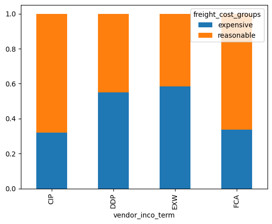
Looks like these two variables are definitely not independent, but let’s test that:

Performing chi squared test

expected, observed, stats = pingouin.chi2_independence(
    data = late_shipments,
    x = "vendor_inco_term",
    y = "freight_cost_groups"
)

stats

	test	lambda	chi2	dof	pval	cramer	power
0	pearson	1.000000	33.642600	3.0	2.357026e-07	0.183511	0.999424
1	cressie-read	0.666667	33.632598	3.0	2.368510e-07	0.183484	0.999423
2	log-likelihood	0.000000	33.895008	3.0	2.084919e-07	0.184198	0.999466
3	freeman-tukey	-0.500000	34.349001	3.0	1.672011e-07	0.185428	0.999533
4	mod-log-likelihood	-1.000000	35.037928	3.0	1.195978e-07	0.187278	0.999620
5	neyman	-2.000000	37.199484	3.0	4.175225e-08	0.192968	0.999802

Finally, we reject the null hypothesis and conclude that these two variables are not independent, they are definitely associated

Chi squared goodness of fit tests

Example 1

This test allows to check if a data proportion fits to your proportion assumption or not.

Example: In the stack overflow dataset, there is a variable called Purple link, this variable measures how users felt when they noticed that clicked the purple link (purple link is literally the first link you get when you google a coding question)

purple_link_counts = (
    stack_overflow["purple_link"]
    .value_counts()
    .rename_axis("purple_link")
    .reset_index(name="n")
    .sort_values("purple_link")
)

purple_link_counts

	purple_link	n
2	Amused	368
3	Annoyed	263
0	Hello, old friend	1225
1	Indifferent	405

that is the original distribution for that answer, which measures what the person felt when noticed that clicked in the purple_link

Declaring Hypothesis

let’s hypothesize that half of the users would respond “Hello, old friend” and the rest would respond the other three options with the same probability

hypothesized = pd.DataFrame({
    "purple_link" : ["Amused", "Annoyed", "Hello, old friend", "Indifferent"],
    "prop" : [1/6, 1/6, 1/2, 1/6]
})

hypothesized

	purple_link	prop
0	Amused	0.166667
1	Annoyed	0.166667
2	Hello, old friend	0.500000
3	Indifferent	0.166667

Like this

Now, our hypotheses would be

\(H_0: \) the sample matches the hypothesized distribution

\(H_1: \) the sample does not match the hypothesized distribution

\(\alpha = 0.01\)

let’s visualize the thing

first we need to know how many responses we would have gotten in our hypothetic distribution, then we will compare that with the sample

n_total = len(stack_overflow)
hypothesized["n"] = hypothesized["prop"] * n_total

hypothesized

	purple_link	prop	n
0	Amused	0.166667	376.833333
1	Annoyed	0.166667	376.833333
2	Hello, old friend	0.500000	1130.500000
3	Indifferent	0.166667	376.833333

plt.bar(
    purple_link_counts["purple_link"],
    purple_link_counts["n"],
    color = "red", label = "Observed"
)

plt.bar(
    hypothesized["purple_link"],
    hypothesized["n"],
    alpha = 0.5,
    color = "blue", label = "Hypothesized"
)

plt.legend()
plt.show()

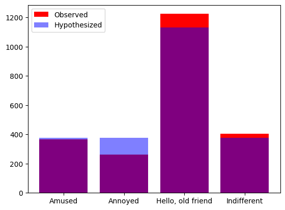
From the chart we can see that “Amused” and “Indifferent” are similar in terms of hypothesized and observed values, but “Annoyed” and “Hello, old friend” seem different.

But, is that difference statistically significant?

Note: this test is called goodness of fit test (PRUEBA DE BONDAD DE AJUSTE) since we are testing how well our hypothesized data fits our actual data

from scipy.stats import chisquare

chisquare(
    f_obs=purple_link_counts["n"],
    f_exp=hypothesized["n"]
)

Power_divergenceResult(statistic=44.59840778416629, pvalue=1.1261810719413759e-09)

Since this p-value is very very small, we reject the null hypothesis and conclude that the sample and the hypothesized distribution are different

Example 2

# Remove that DDU for convenience (it's only one)
late_shipments = late_shipments[late_shipments["vendor_inco_term"] != "DDU"]

incoterm_counts = (
    late_shipments["vendor_inco_term"]
    .value_counts()
    .rename_axis("vendor_inco_term")
    .reset_index(name="n")
    .sort_values("vendor_inco_term")
)

incoterm_counts

	vendor_inco_term	n
3	CIP	56
2	DDP	100
0	EXW	732
1	FCA	111

# Hypothesized ditribution

hypothesized = pd.DataFrame({
    "vendor_inco_term" : ["CIP", "DDP", "EXW", "FCA"],
    "prop" : [0.05, 0.1, 0.75, 0.1]
})

hypothesized

	vendor_inco_term	prop
0	CIP	0.05
1	DDP	0.10
2	EXW	0.75
3	FCA	0.10

# Counts for hypothesized
hypothesized["n"] = hypothesized["prop"] * n_total

# Find the number of rows in late_shipments
n_total = len(late_shipments)

# Create n column that is prop column * n_total
hypothesized["n"] = hypothesized["prop"] * n_total

# Plot a red bar graph of n vs. vendor_inco_term for incoterm_counts
plt.bar(
    incoterm_counts["vendor_inco_term"],
    incoterm_counts["n"],
    color = "red",
    label="Observed")

plt.bar(
    hypothesized['vendor_inco_term'],
    hypothesized['n'],
    alpha = 0.5,
    color="blue", 
    label="Observed")

plt.legend()
plt.show()

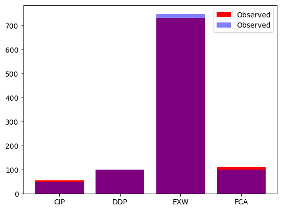
As you can see, the distribution matches a lot with our hypothesized values, but is that similarity statistically significant?

gof_test = chisquare(
    f_obs=incoterm_counts["n"],
    f_exp=hypothesized["n"]
)

gof_test

Power_divergenceResult(statistic=2.3633633633633613, pvalue=0.5004909543758689)

Now, note that this p value greater than our significance level, indicates that we failed to reject the null hypothesis and can conclude that the sample fits well to our hypothesized distribution.

NON Parametric tests

What happens if the assumptions considered in the hypothesis testing are not met?

The tests explained before such as

• z test

• t test

• ANOVA

are parametric tests and are all based on the assumption that the population is normally distributed

Wilcoxon-signed rank test (Paired data)

This test is used for paired data

Given the dataset for election results in the united states for the republicans, let’s hypothesize:

\(H_0:\) Percentage of votes in 2008 is not smaller than 2012

\(H_1:\) Percentage of votes in 2008 is smaller than 2012

repub_votes = pd.read_feather("repub_votes_potus_08_12.feather")

And let’s use a small sample

repub_votes_small = repub_votes.sample(5)

repub_votes_small

	state	county	repub_percent_08	repub_percent_12
78	Texas	Lampasas	74.024103	78.026097
19	Illinois	St. Clair	38.139394	41.957544
32	Kentucky	Jessamine	67.829227	68.981728
72	Tennessee	Chester	71.017185	73.073323
90	Washington	San Juan	28.088501	29.365679

since this data is paired, let’s try to perform a t-test on this small sample (T TEST IS WRONG BECAUSE THERE IS NO NORMALITY, THIS IS JUST TO DO A DEMONSTRATION)

alpha = 0.01

pingouin.ttest(
    x = repub_votes_small["repub_percent_08"],
    y = repub_votes_small["repub_percent_12"],
    paired = True,
    alternative = "less"
)

	T	dof	alternative	p-val	CI95%	cohen-d	BF10	power
T-test	-4.020709	4	less	0.007928	[-inf, -1.16]	0.115798	10.108	0.07693

Basically t-test rejeccts the null hypothesis and suggests that

vote percentages for 2008 are smaller than percentage for 2012

Wicoxon test process

There are many different ways to perform tests without the parametric assumptions, Wilcoxon test is one method related to ranks

from scipy.stats import rankdata

# Creating a list to see it's ranks
x = [1,15,3,10,6]

ranks are the orderings from smallest to largest, scipy.stats allows to access the ranks of a list

rankdata(x)

array([1., 5., 2., 4., 3.])

This tests requires us to calculate the absolute differences in the pairs of data and then rank them

Now, let’s explain how it works…

First, we take differences in the paired values

repub_votes_small["diff"] = repub_votes_small["repub_percent_08"] -  repub_votes_small["repub_percent_12"]

repub_votes_small[["repub_percent_08", "repub_percent_12", "diff"]]

	repub_percent_08	repub_percent_12	diff
78	74.024103	78.026097	-4.001994
19	38.139394	41.957544	-3.818150
32	67.829227	68.981728	-1.152501
72	71.017185	73.073323	-2.056138
90	28.088501	29.365679	-1.277178

Next, we take the absolute value of the differences

repub_votes_small["abs_diff"] = repub_votes_small["diff"].abs()

repub_votes_small[["repub_percent_08", "repub_percent_12", "diff", "abs_diff"]]

	repub_percent_08	repub_percent_12	diff	abs_diff
78	74.024103	78.026097	-4.001994	4.001994
19	38.139394	41.957544	-3.818150	3.818150
32	67.829227	68.981728	-1.152501	1.152501
72	71.017185	73.073323	-2.056138	2.056138
90	28.088501	29.365679	-1.277178	1.277178

Then, we rank these absolute differences

repub_votes_small["rank_abs_diff"] = rankdata(repub_votes_small["abs_diff"])

repub_votes_small[["repub_percent_08", "repub_percent_12", "diff", "abs_diff","rank_abs_diff"]]

	repub_percent_08	repub_percent_12	diff	abs_diff	rank_abs_diff
78	74.024103	78.026097	-4.001994	4.001994	5.0
19	38.139394	41.957544	-3.818150	3.818150	4.0
32	67.829227	68.981728	-1.152501	1.152501	1.0
72	71.017185	73.073323	-2.056138	2.056138	3.0
90	28.088501	29.365679	-1.277178	1.277178	2.0

Finally, we calculate a test statistic called W

W uses the signs of the diff column to split the ranks into two groups:

• One group for rows with negative differences

• One group for rows with positive differences

T_minus is the sum of the ranks with negative differences

print(repub_votes_small[repub_votes_small["diff"] < 0]["rank_abs_diff"])

T_minus = sum (repub_votes_small[repub_votes_small["diff"] < 0]["rank_abs_diff"])

print(T_minus)

78    5.0
19    4.0
32    1.0
72    3.0
90    2.0
Name: rank_abs_diff, dtype: float64
15.0

T_plus is the sum of the ranks with positive differences

print(repub_votes_small[repub_votes_small["diff"] > 0]["rank_abs_diff"])

T_plus = sum (repub_votes_small[repub_votes_small["diff"] > 0]["rank_abs_diff"])

print(T_plus)

Series([], Name: rank_abs_diff, dtype: float64)
0

IN THIS EXAMPLE, ALL THE DIFFERENCES ARE NEGATIVE, SO THE T-MINUS IS THE SUM OF ALL RANKS AND THE T-PLUS IS ZERO.

Now, the test statistic W is the smaller of T-minus and T-plus, in this case it is zero

W = np.min([T_minus, T_plus])

W

0.0

Now, we can calculate W and its corresponding p-value using a pingouin method instead of manual calculation.

pingouin.wilcoxon

alpha = 0.01
pingouin.wilcoxon(
    x = repub_votes_small["repub_percent_08"],
    y = repub_votes_small["repub_percent_12"],
    alternative="less"
)

	W-val	alternative	p-val	RBC	CLES
Wilcoxon	0.0	less	0.03125	-1.0	0.6

Note that the W value returned is the same as our manual calculation

How do we compare this value with the obtained from the T-test?

Remember that t-test rejects the null hypothesis and suggests that

• vote percentages for 2008 are not greater than percentage for 2012

But wilcoxon tells us

• There is not enough evidence that vote percentages for 2008 are smaller than percentages for 2012 using this small sample of five rows

Wilcoxon-Mann-Whitney test (Independent data)

This test works for independent numeric samples

Also known as the Mann Whitney U test

This test also works with ranked data, and it is roughly speaking, a t-test on ranked data

Let’s return to the converted compensation vs the age people began coding

\(H_0:\) Those who code first as children do not have a higher income than those who code first as adults

\(H_1:\) Those who code first as children have a higher income than those who code first as adults

sns.boxplot(
    x = stack_overflow["converted_comp"],
    y = stack_overflow["age_first_code_cut"],
    data = stack_overflow,
    showfliers = False  # removing the outliers just for the chart to look better
)

plt.show()

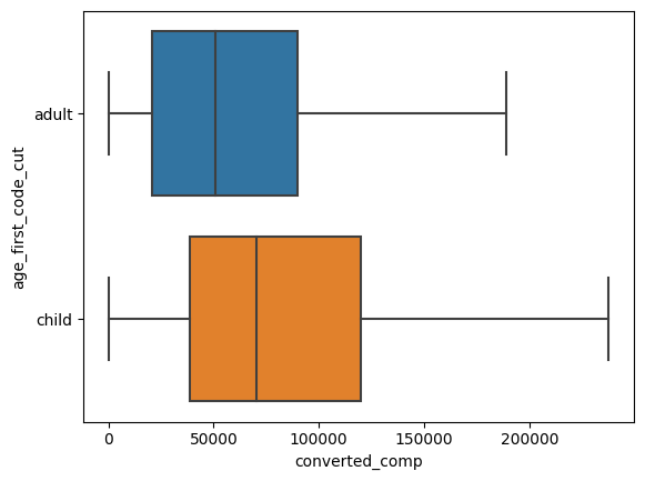
in general, it is visible that people who started coding as childs are better compensated than those who started coding as adults, let’s perform our Wilcoxon-Mann-Whitney test

first, we select just the columns we need:

age_vs_comp = stack_overflow[["converted_comp", "age_first_code_cut"]]

now, to conduct the Wilcoxon-Mann-Whitney test, we need to convert our data from long to wide format

age_vs_comp_wide = age_vs_comp.pivot(columns="age_first_code_cut", values="converted_comp")

age_vs_comp_wide.head()

age_first_code_cut	adult	child
0	77556.0	NaN
1	NaN	74970.0
2	NaN	594539.0
3	2000000.0	NaN
4	37816.0	NaN

alpha = 0.01

pingouin.mwu(
    x = age_vs_comp_wide["child"],
    y = age_vs_comp_wide["adult"],
    alternative = "greater"
)

	U-val	alternative	p-val	RBC	CLES
MWU	744365.5	greater	1.902723e-19	-0.222516	0.611258

With this very small p-value, we can be sure that people who started coding as childs, earn more money

Kruskal-Wallis test

Kruskal-Wallist test is to Wilcoxon-Mann-Whitney test

as

ANOVA is to t-test

Meaning, this is the non parametric way to test a numeric variable across more than two groups.

That is The Kruskall-Wallis test is the non parametric version of ANOVA

let’s use this test to see if there is a difference in converted_comp between job satisfaction groups

sns.boxplot(
    x = stack_overflow["converted_comp"],
    y = stack_overflow["job_sat"],
    data = stack_overflow,
    showfliers = False  # removing the outliers just for the chart to look better
)

plt.show()

alpha = 0.01

pingouin.kruskal(
    data = stack_overflow,
    dv = "converted_comp",
    between = "job_sat"
)

	Source	ddof1	H	p-unc
Kruskal	job_sat	4	72.814939	5.772915e-15

The p-value is very smaller than our significance level, this provides evidence that at least one of the mean compensation totals is different than the others across these five job satisfaction groups

Created in Deepnote